PPO

I thought PPO is so daunting as it’s used by every LLM and some robotics frontier research. It turns out it’s actually much simpler than TRPO, just like how GRPO is simpler than PPO.

The paper itself is easy to read. Other than that there’s also OpenAI Spinning up which offers simpler formulas (why don’t they include that in the paper? I derived them myself anyway since it was confusing) and explanations, and the A Primer on LLM Post-Training on PyTorch blog. Note that blog contains invalid opinions, e.g. when explaining why there’s the min in the PPO formula. I think the author confuses themselves.

Anyway, let’s get started!

---

The following note come from my conversation with Claude Sonnet 4.6

---

PPO asks the same question as TRPO: how do we take the biggest possible improvement step without accidentally collapsing performance? Where TRPO answers with complex second-order machinery, PPO is a family of first-order methods that enforce the trust region through the loss function shape itself — no Fisher matrix, no conjugate gradient, just plain SGD/Adam.

There are two variants: PPO-Clip (primary) and PPO-Penalty (adaptive KL). This note focuses on PPO-Clip.

Where the trust region comes from: CPI → TRPO → PPO

The whole family rests on one bound from Conservative Policy Iteration (Kakade & Langford, 2002) — this is what the superscript in $L^{CPI}$ refers to. CPI’s original move was to update the policy conservatively, mixing ${\pi }_{new}=(1-\alpha ){\pi }_{old}+\alpha {\pi }^{\prime }$ instead of greedily replacing it, so the state distribution can’t lurch in one step. TRPO later recast that idea in KL terms as a bound:

$$\eta (\pi )\ge L^{CPI}(\pi )-C\underset{s}{\max }\mathrm{KL}[{\pi }_{{\theta }_k}(\cdot |s)\Vert \pi (\cdot |s)]$$

• $\eta (\pi )$ is the true return — what you’d actually measure by running $\pi$ in the environment. Computing it exactly needs fresh on-policy rollouts from $\pi$ itself, which you don’t have mid-update.
• $L^{CPI}(\pi )={\mathbb{E}}_{{\pi }_{{\theta }_k}}[r_t{\hat{A}}_t]$ is the surrogate — computable from the frozen batch, but only trustworthy near ${\pi }_{{\theta }_k}$ (it reweights the action distribution via $r_t$ but ignores the state-distribution shift the new policy would cause).
• The bound quantifies exactly how far the surrogate can drift from the truth, as a function of how much the policy moved. Maximize the RHS and true improvement is guaranteed — that’s the whole reason to keep $\pi$ close to ${\pi }_{{\theta }_k}$.

Note it’s ${\max }_s$ KL, not mean — a genuine worst-case/pessimistic bound, since a single state where the policy lurches can blow up the true gap. TRPO already softens this to mean KL in practice (the max is intractable), the first of several places theory gets traded for tractability.

Penalty vs. constraint — and why you can't just solve for β

The bound is literally a penalty: maximize $L^{CPI}-\beta \mathrm{KL}$. That’s an unconstrained Lagrangian, with $\beta$ the multiplier on a KL constraint. Duality says some ${\beta }^{\ast }$ reproduces any hard KL-radius $\delta$ exactly — so in theory penalty and constraint are equivalent. In practice you can’t pick ${\beta }^{\ast }$ in closed form:

• It depends on the local curvature of KL (the Fisher matrix) around ${\theta }_k$, which shifts as training moves through parameter space.
• It depends on the scale of the advantages — raw reward-derived units, wildly different across tasks (rewards in $[-1,1]$ vs. the thousands).
• So a $\beta$ tuned early is the wrong $\beta$ later, within a single run.

This is exactly why TRPO uses a hard constraint (maximize $L^{CPI}$ s.t. $\overline{\mathrm{KL}}\le \delta$), enforced numerically with conjugate gradient + line search — it never has to guess $\beta$. PPO-Penalty instead keeps the penalty form but makes $\beta$ adaptive. PPO-Clip drops the KL machinery entirely and gets the trust-region effect from the loss shape instead.

The Clipped Surrogate Objective

Let $r_t(\theta )=\frac{{\pi }_{\theta }(a_t|s_t)}{{\pi }_{{\theta }_k}(a_t|s_t)}$ be the probability ratio. ${\theta }_k$ is the frozen behavioral policy — the parameters that generated the current rollout batch ${\mathcal{D}}_k$; it stays pinned throughout all inner SGD epochs, with $k$ only incrementing when new trajectories are collected. The raw (unclipped) surrogate is just $r_t{A}_t$ — this is $L^{CPI}$, the policy gradient objective with importance sampling.

The PPO-Clip objective is:

$$L^{CLIP}(\theta )={\hat{\mathbb{E}}}_t\left[\min \left(r_t(\theta ){\hat{A}}_t,g(ϵ,{\hat{A}}_t)\right)\right]$$

where the clipping function is:

$$g(ϵ,A)=\{\begin{array}{ll}(1+ϵ)A& A\ge 0\\ (1-ϵ)A& A<0\end{array}$$

This simplified form (from SpinningUp) is equivalent to the original paper’s $\min (r_t{A}_t,\text{clip}(r_t,1-ϵ,1+ϵ)A_t)$ but makes the intent clearer.

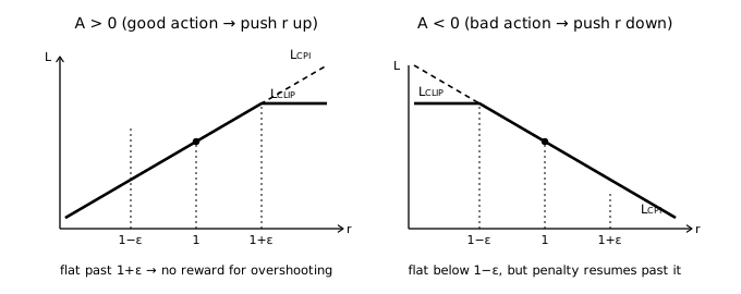
The shape is the whole idea: the objective tracks the unclipped line $r_t{A}_t$ near $r=1$ (the dot), then goes flat on the side where more movement would help — so there’s no gradient reward for pushing past the band. On the side where more movement would hurt, the line (penalty) stays live.

Why min() on top of clipping?

Clipping alone just flatlines the objective at the boundary — it stops rewarding further movement, but doesn’t penalize overshooting. The min() makes it a pessimistic lower bound: it reintroduces the worse (unclipped) value whenever you’ve moved so far that it’s worse than the clipped version. The two cases make this concrete:

When $A_t>0$ (action was good, increase its probability):

• Past $(1+ϵ)$, the clipped term flatlines
• The unclipped term keeps growing — so min = clipped (flatline) ✓
• No gradient incentive to keep pushing $r_t$ above $1+ϵ$

When $A_t<0$ (action was bad, decrease its probability):

• Past $(1-ϵ)$, the clipped term flatlines
• The unclipped term keeps getting more negative — so min = unclipped (penalty) ✓
• Overshoot is still penalized even though you’re outside the clip band

Equivalently, you could write it with a conditional — only clip the side that would let the objective keep improving:

$$L_t=\{\begin{array}{ll}\min (r_t,1+ϵ),A_t& A_t>0\\ \max (r_t,1-ϵ),A_t& A_t<0\end{array}$$

The min() formulation is just a branchless way to express this.

On the notation $L$: it’s a pseudo-loss

$L^{CLIP}$, $L^{CPI}$, etc. are surrogate objectives, not the true RL objective. The true objective is the expected return $J(\theta )$; $L$ is a differentiable stand-in whose gradient is engineered to point in a useful direction. Optimizers minimize, so in code the policy “loss” is the negated batch mean of the surrogate:

$$L_{\text{policy}}=-\frac{1}{N}\sum _t\min (r_t{\hat{A}}_t,g(ϵ,{\hat{A}}_t))$$

The mathematical object has an expectation ${\hat{\mathbb{E}}}_t$; the minibatch mean is just its Monte Carlo estimate.

Why no REINFORCE log-derivative trick here?

The whole reason REINFORCE needs the trick is that its expectation is taken over ${\pi }_{\theta }$ itself — the sampling distribution depends on the very parameters we differentiate. You can’t push ${\nabla }_{\theta }$ through ${\mathbb{E}}_{a\sim {\pi }_{\theta }}[\cdot ]$ directly, so you rewrite ${\nabla }_{\theta }{\pi }_{\theta }={\pi }_{\theta }{\nabla }_{\theta }\log {\pi }_{\theta }$ to turn the gradient back into an expectation you can sample.

PPO’s surrogate is an expectation over the frozen ${\pi }_{{\theta }_k}$ (see Importance sampling corrections):

$L^{CPI}(\theta )={\mathbb{E}}_{(s,a)\sim {\pi }_{{\theta }_k}}\left[r_t(\theta ){\hat{A}}_t\right]$

The distribution we sample from does not depend on $\theta$. So we can just sample directly and move the gradient inside — no trick needed:

${\nabla }_{\theta }{L}^{CPI}={\mathbb{E}}_{{\pi }_{{\theta }_k}}\left[{\hat{A}}_t{\nabla }_{\theta }{r}_t(\theta )\right]$

That’s the conceptual leap from on-policy PG to importance-sampled surrogates: fix the sampling distribution first, then correct the mismatch with the ratio $r_t$.

The score function reappears anyway

Even though we never invoke the trick, differentiating the ratio reconstructs it. Since $r_t=\exp (\log {\pi }_{\theta }-\log {\pi }_{{\theta }_k})$ and ${\pi }_{{\theta }_k}$ is constant, ${\nabla }_{\theta }{r}_t=r_t{\nabla }_{\theta }\log {\pi }_{\theta }$. Evaluated at $\theta ={\theta }_k$ where $r_t=1$, the surrogate gradient collapses to $\mathbb{E}[{\hat{A}}_t{\nabla }_{\theta }\log {\pi }_{\theta }]$ — exactly the policy gradient. So PPO’s gradient equals vanilla PG in a neighborhood of ${\theta }_k$; clipping only changes what happens once the inner SGD epochs drift $r_t$ far from 1.

(Aside: the exp(logp_new - logp_old) in code is not logits→probabilities — that’s softmax. It’s recovering the probability ratio ${\pi }_{\theta }/{\pi }_{{\theta }_k}$ from log-probs in a numerically stable way.)

Why This Works Better Than TRPO in Practice

• See Limitations of TRPO

But TRPO has monotonic improvement guarantees — how can PPO beat it?

The theoretical bound is extremely loose. What matters empirically is “does this update move in a good direction without destabilizing training?” Clipping is a robust heuristic for this. PPO also benefits from the multiple SGD epochs squeezing more signal from each batch of environment data, which TRPO simply can’t do. The complexity TRPO pays for its guarantee buys very little in practice. I pressed Sonnet 4.6 really hard and it admit it’s all empirical.

Why can PPO run multiple SGD epochs on one batch, but TRPO can't?

Not spelled out in the paper, but the reason is structural. TRPO builds each update from a one-shot local approximation: it linearizes $L^{CPI}$ and puts a quadratic (Fisher) model on the KL, both expanded around ${\theta }_k$, then solves that subproblem once via conjugate gradient + line search. After a single step those Taylor expansions are stale — to step again you’d have to re-linearize and re-run CG, which is a whole new TRPO update, not a cheap extra epoch.

PPO-Clip’s objective is the exact nonlinear function of $\theta$ everywhere — nothing is expanded around ${\theta }_k$, only the frozen ${\pi }_{{\theta }_k}$ in the denominator of $r_t$ is fixed. So you can take Adam step after Adam step on the same batch, recomputing $r_t(\theta )$ each time; the clip keeps every step honest because the flat region lives in the objective’s shape at every $\theta$, not in a local model that expires after one step. This off-policy reuse is what the importance ratio is for — the clip is just the safety valve that stops the reuse from drifting too far (paper uses ~3–15 epochs).

PPO-Penalty (Adaptive KL)

Instead of clipping, penalize KL directly:

$$L^{KLPEN}(\theta )={\hat{\mathbb{E}}}_t\left[r_t{\hat{A}}_t-\beta \cdot D_{KL}[{\pi }_{{\theta }_k}|{\pi }_{\theta }]\right]$$

$\beta$ is adjusted each update:

• If $KL>1.5,\delta$: increase $\beta$
• If $KL<\delta /1.5$: decrease $\beta$
• Otherwise: leave it

Note

This is basically bang-bang control with a deadband — a discrete switching rule on threshold crossings. The paper admits $\beta$-tuning is fiddly, and PPO-Clip empirically outperforms this variant. The more principled version of adaptive $\lambda$ is dual gradient descent (gradient ascent on the Lagrange multiplier), which has actual convergence theory and shows up in constrained RL (CMDPs) and RLHF KL tuning.

Entropy Bonus

The full objective often adds an entropy term:

$$L=L^{CLIP}-c_1{L}^{VF}+c_{2}H[{\pi }_{\theta }]$$

where $H[{\pi }_{\theta }]=-{\sum }_a{\pi }_{\theta }(a|s)\log {\pi }_{\theta }(a|s)$.

This prevents policy collapse — gradient descent naturally wants to concentrate probability on the best-so-far action, which kills exploration. High entropy = spread distribution (exploratory). The entropy bonus penalizes overconfident policies, keeping exploration alive longer.

This is the same regularization intuition as load balancing loss in Mixture of Experts: the primary objective has no incentive to maintain diversity, so you add a term that explicitly fights the degenerate low-entropy solution. The difference is what “collapse” means — MoE collapses across experts for a token; policy gradient collapses across actions for a state.

Advantage estimation: truncated GAE

The algorithm box below says “any method of advantage estimation” — in practice that’s truncated GAE, and the “truncated” part is what makes PPO’s rollout loop work. Rather than waiting for an episode to terminate before you can compute ${\hat{A}}_t$, you run the policy for a fixed $T$ steps ($T\ll$ episode length) and bootstrap the unseen future with the value function:

$${\hat{A}}_t=-V(s_t)+r_t+\gamma r_{t+1}+\cdots +{\gamma }^{T-t-1}{r}_{T-1}+\underset{\text{bootstrap at the cutoff}}{\underbrace{{\gamma }^{T-t}V(s_T)}}$$

That last term is the whole trick: it stands in for “everything after $T$,” so you can update from a $T$-step segment without ever seeing the episode end. This is what lets PPO (a) train recurrent policies on fixed-length contiguous segments, and (b) update frequently on long or non-episodic tasks. The formula above is the $\lambda =1$ special case; general GAE blends every within-window $n$-step estimator, ${\hat{A}}_t={\sum }_l(\gamma \lambda {)}^l{\delta }_{t+l}$ with ${\delta }_t=r_t+\gamma V(s_{t+1})-V(s_t)$.

What GAE buys over a fixed n-step TD return

Both are the MC↔TD dial; GAE just refuses to commit to one $n$. An $n$-step return forces a hard cutoff — step $n$ is “real reward,” step $n+1$ is bootstrapped away, an artificial discontinuity. GAE instead takes an exponentially-weighted average of all $n$-step estimators, so influence fades gradually. Concretely:

• One continuous, transferable knob $\lambda \in [0,1]$ instead of an integer $n$ whose “right” value swings by orders of magnitude across environments (5 vs. 500). $\lambda \in [0.9,0.99]$ works almost everywhere.
• Graceful degradation — a bad $n$ can wreck an estimator; GAE isn’t betting everything on one horizon, so it’s robust to the value function being mediocre early in training.

Cost is a cheap linear-time backward pass over the segment. $n$-step TD (any $n$) and Monte Carlo are literally its $\lambda \to 0$ and $\lambda \to 1$ limits.

\begin{algorithm}
\begin{algorithmic}
\REQUIRE initial policy parameters $\theta_{0}$, initial value function parameters $\phi_{0}$
\FOR{$k = 0, 1, 2, \dots$}
    \STATE Collect set of trajectories $\mathcal{D}_{k} = \{\tau_{i}\}$ by running policy $\pi_{k} = \pi(\theta_{k})$ in the environment.
    \STATE Compute rewards-to-go $\hat{R}_{t}$.
    \STATE Compute advantage estimates, $\hat{A}_{t}$ (using any method of advantage estimation) based on the current value function $V_{\phi_{k}}$.
    \STATE Update the policy by maximizing the PPO-Clip objective:
    \STATE $$\theta_{k+1} = \arg \max_{\theta} \frac{1}{|\mathcal{D}_{k}|T} \sum_{\tau \in \mathcal{D}_{k}} \sum_{t=0}^{T} \min \left( \frac{\pi_{\theta}(a_{t}|s_{t})}{\pi_{\theta_{k}}(a_{t}|s_{t})} A^{\pi_{\theta_{k}}}(s_{t}, a_{t}), g(\epsilon, A^{\pi_{\theta_{k}}}(s_{t}, a_{t})) \right)$$
    \STATE \textit{typically via stochastic gradient ascent with Adam.}
    \STATE Fit value function by regression on mean-squared error:
    \STATE $$\phi_{k+1} = \arg \min_{\phi} \frac{1}{|\mathcal{D}_{k}|T} \sum_{\tau \in \mathcal{D}_{k}} \sum_{t=0}^{T} \left( V_{\phi}(s_{t}) - \hat{R}_{t} \right)^{2}$$
    \STATE \textit{typically via some gradient descent algorithm.}
\ENDFOR
\end{algorithmic}
\end{algorithm}

The honest read: clip is a heuristic, not a theorem

Worth remembering when the mystique wears off: the paper never proves $L^{CLIP}$ inherits the monotonic-improvement guarantee that justified the whole CPI/TRPO trust-region story. The only formal claim it makes about the clip is a single sentence in Section 3, right after eq. (7):

$L^{CLIP}(\theta )=L^{CPI}(\theta )$ to first order around ${\theta }_{old}$ (i.e., where $r=1$) … they become different as $\theta$ moves away from ${\theta }_{old}$.

That’s asserted, not derived — but it’s easy to verify: at ${\theta }_k$ every $r_t=1$, sitting at the center of the clip band where clip is the identity, so $L^{CLIP}$ and $L^{CPI}$ (and their gradients) coincide in a neighborhood. It’s the same fact the score-function callout uses to show PPO’s gradient equals vanilla policy gradient near ${\theta }_k$. Everything past first order is empirical: $ϵ=0.2$, “clip the ratio not log-space” (they tried log-space, report “no better,” and say nothing more), the epoch count — all justified by the Table 1 ablation across 7 MuJoCo tasks, not by a bound. So yes: the honest one-line summary is “this is plausible given TRPO’s backdrop, we tried it, it works great, and we’re not going to prove it.” Characteristic of that era of deep RL — TRPO is the rigorous one; PPO explicitly trades the rigor for simplicity and empirical performance, which is the stated goal in the abstract.