Actor-Critic

The source material is CS285, 2023, with some 2026 lecture note sprinkled in.

Actor-Critic is letting the network output its estimation of $Q$ or $V$, combining with Policy Gradient, so that it’s no longer a Monte Carlo update, smaller variance.

Recall REINFORCE with baseline:

$${\nabla }_{\theta }J(\theta )\approx \frac{1}{N}\sum _{i=1}^N\sum _{t=1}^T{\nabla }_{\theta }\log {\pi }_{\theta }({\mathbf{a}}_{i,t}|{\mathbf{s}}_{i,t})(Q({\mathbf{s}}_{i,t},{\mathbf{a}}_{i,t})-b)$$

A good choice of $b$ is simply $V({\mathbf{s}}_t)=E_{{\mathbf{a}}_t\sim {\pi }_{\theta }({\mathbf{a}}_t|{\mathbf{s}}_t)}[Q({\mathbf{s}}_t,{\mathbf{a}}_t)]$. We can then define the Advantage: how much better $a_t$ is, compare with the state average:

$$\begin{array}{rl}{A}^{\pi }({\mathbf{s}}_t,{\mathbf{a}}_t)& =Q^{\pi }({\mathbf{s}}_t,{\mathbf{a}}_t)-V^{\pi }({\mathbf{s}}_t)\\ {\nabla }_{\theta }J(\theta )& \approx \frac{1}{N}\sum _{i=1}^N\sum _{t=1}^T{\nabla }_{\theta }\log {\pi }_{\theta }({\mathbf{a}}_{i,t}|{\mathbf{s}}_{i,t})A^{\pi }({\mathbf{s}}_{i,t},{\mathbf{a}}_{i,t})\end{array}$$

We commonly have the network fit $V^{\pi }$ instead of $Q^{\pi }$ or $A^{\pi }$, as it depend just on state and doesn’t need so many samples to learn, and

$$\begin{array}{rl}{Q}^{\pi }({\mathbf{s}}_t,{\mathbf{a}}_t)& =r({\mathbf{s}}_t,{\mathbf{a}}_t)+E_{{\mathbf{s}}_{t+1}\sim p({\mathbf{s}}_{t+1}|{\mathbf{s}}_t,{\mathbf{a}}_t)}[V^{\pi }({\mathbf{s}}_{t+1})]\\ & \approx r({\mathbf{s}}_t,{\mathbf{a}}_t)+V^{\pi }({\mathbf{s}}_{t+1})\\ A^{\pi }({\mathbf{s}}_t,{\mathbf{a}}_t)& \approx r({\mathbf{s}}_t,{\mathbf{a}}_t)+V^{\pi }({\mathbf{s}}_{t+1})-V^{\pi }({\mathbf{s}}_t)\end{array}$$

That approximation is to use the state taken by our policy this round as the expected next state by our policy.

Evaluation (getting V)

That’s basically value based method. We can use Monte Carlo or Temporal difference and estimating $V$ is a supervised learning problem.

With TD the training pair is basically bootstrapping:

$$\left\{\left({\mathbf{s}}_{i,t},r({\mathbf{s}}_{i,t},{\mathbf{a}}_{i,t})+{\hat{V}}_{\varphi }^{\pi }({\mathbf{s}}_{i,t+1})\right)\right\}$$

You can see stuff about this in Function approximation, that one is from the DeepMind / UCL 2021 course.

\begin{algorithm}
\caption{Batch Actor-Critic Algorithm}
\begin{algorithmic}
\WHILE{TRUE}
    \STATE 1. sample $\{\mathbf{s}_i, \mathbf{a}_i\}$ from $\pi_\theta(\mathbf{a}|\mathbf{s})$ (run it on the robot)
    \STATE 2. fit $\hat{V}_\phi^\pi(\mathbf{s})$ to sampled reward sums
    \STATE 3. evaluate $\hat{A}^\pi(\mathbf{s}_i, \mathbf{a}_i) = r(\mathbf{s}_i, \mathbf{a}_i) + \gamma\hat{V}_\phi^\pi(\mathbf{s}'_i) - \hat{V}_\phi^\pi(\mathbf{s}_i)$
    \STATE 4. $\nabla_\theta J(\theta) \approx \sum_i \nabla_\theta \log \pi_\theta(\mathbf{a}_i|\mathbf{s}_i)\hat{A}^\pi(\mathbf{s}_i, \mathbf{a}_i)$
    \STATE 5. $\theta \leftarrow \theta + \alpha \nabla_\theta J(\theta)$
\ENDWHILE
\end{algorithmic}
\end{algorithm}

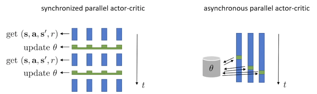
More on on policy actor-critic

It Can be two network or shared network.

Off-policy actor-critic

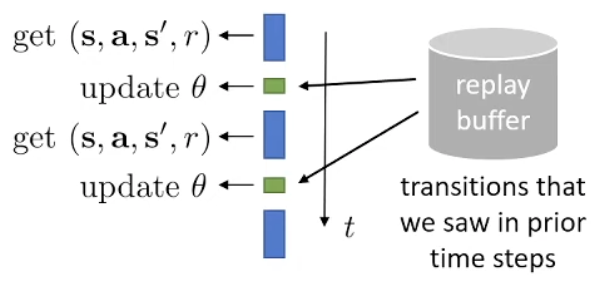But there’s more! To convert on-policy algorithm to off-policy we normally use Importance sampling corrections, but there are easier way to do it here.

Let’s first review the (wrong) online actor-critic algorithm:

\begin{algorithm}
\caption{Wrong Online Actor-critic}
\begin{algorithmic}
\WHILE{not converged}
    \STATE 1. Take action $a \sim \pi_{\theta}(a|s)$, get $(s, a, s', r)$, store in $\mathcal{R}$
    \STATE 2. Sample a batch $\{s_i, a_i, r_i, s'_i\}$ from buffer $\mathcal{R}$
    \STATE 3. Update $\hat{V}_{\phi}^{\pi}$ using targets $y_i = \mathbf{r_i + \gamma \hat{V}_{\phi}^{\pi}(s'_i)}$ \COMMENT{Target Value Issue}
    \STATE 4. Evaluate $\hat{A}^{\pi}(s_i, a_i) = r(s_i, a_i) + \gamma \hat{V}_{\phi}^{\pi}(s'_i) - V_{\phi}^{\pi}(s_i)$
    \STATE 5. $\nabla_{\theta}J(\theta) \approx \frac{1}{N} \sum_i \mathbf{\nabla_{\theta} \log \pi_{\theta}(a_i|s_i)} \hat{A}^{\pi}(s_i, a_i)$ \COMMENT{Action Mismatch Issue}
    \STATE 6. $\theta \leftarrow \theta + \alpha \nabla_{\theta}J(\theta)$
\ENDWHILE
\end{algorithmic}
\end{algorithm}

• We evaluate how good a state is based on $\pi$, and that’s not our current $\pi$. What doesn’t depend on $\pi$ is $Q(s_t,a_t)$, in the sense that the $a_t$ is picked and does not depend on a specific $\pi$, it’s just later in the sequence we follow $\pi$. So… we can make step 3 “on policy”, by sampling a $a_i^{\prime }$ from current policy, not from replay buffer $\mathcal{R}$. If I found myself in the situation $s_i$ and took action $a_i$ (as I did in the past), but then switched to my current strategy for all future steps, what would my total reward be?
• Similarly, we can make step 5 “on policy”, by using $a_i^{\pi }$ instead of $a_i$. We can also for convenience, just use ${\hat{Q}}^{\pi }$ instead of ${\hat{A}}^{\pi }$, higher variance but ok. So now we don’t need $\hat{V}$ any more. It’s okay since we can now just generate more samples.

\begin{algorithm}
\caption{Off-Policy Actor-Critic with Experience Replay}
\begin{algorithmic}
\WHILE{training}
    \STATE 1. take action $\mathbf{a} \sim \pi_{\theta}(\mathbf{a}|\mathbf{s})$, get $(\mathbf{s}, \mathbf{a}, \mathbf{s}', r)$, store in $\mathcal{R}$
    \STATE 2. sample a batch $\{\mathbf{s}_i, \mathbf{a}_i, r_i, \mathbf{s}'_i\}$ from buffer $\mathcal{R}$
    \STATE 3. update $\hat{Q}_{\phi}^{\pi}$ using targets $y_i = r_i + \gamma \hat{Q}_{\phi}^{\pi}(\mathbf{s}'_i, \mathbf{a}'_i)$ for each $\mathbf{s}_i, \mathbf{a}_i$
    \STATE 4. $\nabla_{\theta} J(\theta) \approx \frac{1}{N} \sum_{i} \nabla_{\theta} \log \pi_{\theta}(\mathbf{a}_i^{\pi}|\mathbf{s}_i) \hat{Q}^{\pi}(\mathbf{s}_i, \mathbf{a}_i^{\pi})$ where $\mathbf{a}_i^{\pi} \sim \pi_{\theta}(\mathbf{a}|\mathbf{s}_i)$
    \STATE 5. $\theta \leftarrow \theta + \alpha \nabla_{\theta} J(\theta)$
\ENDWHILE
\end{algorithmic}
\end{algorithm}

Take a closer look, the replay buffer is basically just used for getting the $Q$ part for policy gradient. Off policy critic, on policy actor.

We can use a reparametrization trick. Covered later.

Critics as Baselines

Well, initially we just want a baseline. And somehow we estimate the whole $Q$ or $A$ or $V$. So now it can be biased. There exist a middle ground, still monte carlo rollout, but just use our estimation as the baseline, not the whole $Q$.

$${\nabla }_{\theta }J(\theta )\approx \frac{1}{N}\sum _{i=1}^N\sum _{t=1}^T{\nabla }_{\theta }\log {\pi }_{\theta }({\mathbf{a}}_{i,t}|{\mathbf{s}}_{i,t})\left(\left(\sum _{t^{\prime }=t}^T{\gamma }^{t^{\prime }-t}r({\mathbf{s}}_{i,t^{\prime }},{\mathbf{a}}_{i,t^{\prime }})\right)-{\hat{V}}_{\varphi }^{\pi }({\mathbf{s}}_{i,t})\right)$$

Here the baseline only depend on $s$. If we want to let it be action-dependent, it’s called control variates, discussed in Q-Prop paper.

The core idea is this:

$${\hat{A}}^{\pi }({\mathbf{s}}_t,{\mathbf{a}}_t)=\sum _{t^{\prime }=t}^{\infty }{\gamma }^{t^{\prime }-t}r({\mathbf{s}}_{t^{\prime }},{\mathbf{a}}_{t^{\prime }})-V_{\varphi }^{\pi }({\mathbf{s}}_t)$$

• No bias
• Higher variance

$${\hat{A}}^{\pi }({\mathbf{s}}_t,{\mathbf{a}}_t)=\sum _{t^{\prime }=t}^{\infty }{\gamma }^{t^{\prime }-t}r({\mathbf{s}}_{t^{\prime }},{\mathbf{a}}_{t^{\prime }})-Q_{\varphi }^{\pi }({\mathbf{s}}_t,{\mathbf{a}}_t)$$

• Goes to zero in expectation if critic is correct
• Not correct, doesn’t make sense

So it’s shown that the math work out like follows, note there’s an extra term to compensate for use using that $Q$ in baseline.

$${\nabla }_{\theta }J(\theta )\approx \frac{1}{N}\sum _{i=1}^N\sum _{t=1}^T{\nabla }_{\theta }\log {\pi }_{\theta }({\mathbf{a}}_{i,t}|{\mathbf{s}}_{i,t})\left({\hat{Q}}_{i,t}-Q_{\varphi }^{\pi }({\mathbf{s}}_{i,t},{\mathbf{a}}_{i,t})\right)-\frac{1}{N}\sum _{i=1}^N\sum _{t=1}^T{\nabla }_{\theta }{\mathbb{E}}_{\mathbf{a}\sim {\pi }_{\theta }({\mathbf{a}}_t|{\mathbf{s}}_{i,t})}\left[Q_{\varphi }^{\pi }({\mathbf{s}}_{i,t},{\mathbf{a}}_t)\right]$$

Generalized advantage estimation

A paper by Sculman, Moritz, Levine, Jordan, Abbeel

This provide a better way of estimating ${\hat{A}}^{\pi }$ in on-policy actor critic (not simple TD).

Recall the idea of n-step return from Temporal difference. We can have a weighted combination of these returns, instead of just choosing one of them.

$${\hat{A}}_{\text{GAE}}^{\pi }({\mathbf{s}}_t,{\mathbf{a}}_t)=\sum _{n=1}^{\infty }{w}_n{\hat{A}}_n^{\pi }({\mathbf{s}}_t,{\mathbf{a}}_t)$$

If you think closer, n-step return are already weighted internally by $\gamma$. So we are basically introducing a new term (prefer cutting earlier) for decaying. Say we use exponential falloff, $w_n\propto {\lambda }^{n-1}$, then we can just get…

$$\begin{array}{rl}{\hat{A}}_{\text{GAE}}^{\pi }({\mathbf{s}}_t,{\mathbf{a}}_t)& =r({\mathbf{s}}_t,{\mathbf{a}}_t)+\gamma ((1-\lambda ){\hat{V}}_{\varphi }^{\pi }({\mathbf{s}}_{t+1})+\lambda (r({\mathbf{s}}_{t+1},{\mathbf{a}}_{t+1})+\gamma ((1-\lambda ){\hat{V}}_{\varphi }^{\pi }({\mathbf{s}}_{t+2})+\lambda r({\mathbf{s}}_{t+2},{\mathbf{a}}_{t+2})+\dots )\\ {\hat{A}}_{\text{GAE}}^{\pi }({\mathbf{s}}_t,{\mathbf{a}}_t)& =\sum _{t^{\prime }=t}^{\infty }(\gamma \lambda {)}^{t^{\prime }-t}{\delta }_{t^{\prime }}{\delta }_{t^{\prime }}=r({\mathbf{s}}_{t^{\prime }},{\mathbf{a}}_{t^{\prime }})+\gamma {\hat{V}}_{\varphi }^{\pi }({\mathbf{s}}_{t^{\prime }+1})-{\hat{V}}_{\varphi }^{\pi }({\mathbf{s}}_{t^{\prime }})\end{array}$$

This is the first part of implementing PPO

\begin{algorithm}
\caption{Policy Gradient with GAE}
\begin{algorithmic}
\WHILE{not converged}
    \STATE 1. Sample trajectories $\{\tau^{(i)}\}$ from $\pi_\theta$ (run the policy)
    \STATE 2. Evaluate targets $y_t^{(i)} = r(\mathbf{s}_t^{(i)}, \mathbf{a}_t^{(i)}) + \gamma \hat{V}_\phi^\pi(\mathbf{s}_{t+1}^{(i)})$
    \STATE 3. Fit $\hat{V}_\phi^\pi(\mathbf{s})$ to targets $\{y_t^{(i)}\}$
    \STATE 4. Evaluate $\hat{A}_{\text{GAE}}^\pi(\mathbf{s}_t^{(i)}, \mathbf{a}_t^{(i)}) = \sum_{t'=t}^\infty (\gamma \lambda)^{t'-t} \delta_{t'}^{(i)}$
    \STATE 5. Center and normalize the advantages:
    \STATE $\quad \mu = \frac{1}{HN} \sum_{i,t} \hat{A}^\pi(\mathbf{s}_t^{(i)}, \mathbf{a}_t^{(i)})$
    \STATE $\quad \sigma = \sqrt{\frac{1}{HN} \sum_{i,t} (\hat{A}^\pi(\mathbf{s}_t^{(i)}, \mathbf{a}_t^{(i)}) - \mu)^2}$
    \STATE $\quad \bar{A}^\pi(\mathbf{s}_t^{(i)}, \mathbf{a}_t^{(i)}) = \frac{\hat{A}^\pi(\mathbf{s}_t^{(i)}, \mathbf{a}_t^{(i)}) - \mu}{\sigma}$
    \STATE 6. Estimate gradient $\nabla_\theta J(\theta) \approx \sum_i \sum_t \nabla_\theta \log \pi_\theta(\mathbf{a}_t^{(i)}|\mathbf{s}_t^{(i)}) \bar{A}^\pi(\mathbf{s}_t^{(i)}, \mathbf{a}_t^{(i)})$
    \STATE 7. Update policy $\theta \leftarrow \theta + \alpha \nabla_\theta J(\theta)$
\ENDWHILE
\end{algorithmic}
\end{algorithm}