Deformable DETR

---

Note from my discussion with Claude Opus 4.7, drafted by Sonnet 4.6

---

Paper: Deformable DETR (Zhu et al., 2020), §4.1.

Core insight

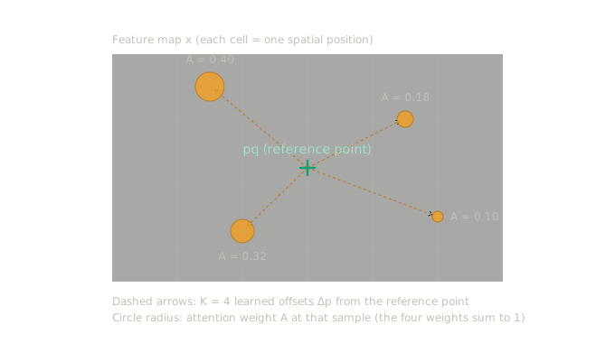
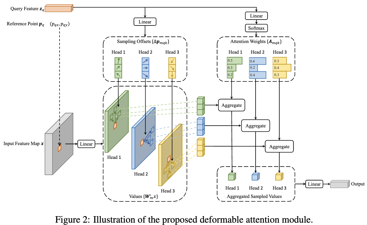
Instead of attending to every spatial location (cost $O(H^2{W}^2)$), each query learns K spatial offsets from a reference point and only attends to those K locations. Offsets and weights both come from the query alone — no query-key dot product.

The formula (single-scale)

$$\text{DeformAttn}(z_q,p_q,x)=\sum _{m=1}^M{W}_m\left[\sum _{k=1}^K{A}_{mqk}\cdot W_m^{\prime }\cdot x(p_q+\Delta p_{mqk})\right]$$

Symbol	Meaning
$z_q$	Query feature vector ($C$-dim)
$p_q$	Reference point (2D coordinate)
$x$	Feature map ($C\times H\times W$)
$m$	Head index ($M$ heads, default 8)
$k$	Sample index ($K$ per head, default 4)
$\Delta p_{mqk}$	Sampling offset (2D, unconstrained range)
$A_{mqk}$	Attention weight; ${\sum }_k{A}_{mqk}=1$ per head
$W_m^{\prime }$	Value projection matrix (per head)
$W_m$	Output projection matrix (per head)

How offsets and weights are computed

Both $\Delta p_{mqk}$ and $A_{mqk}$ come from a single linear projection on $z_q$ with $3MK$ output channels:

• First $2MK$ channels → reshape to $(M,K,2)$ → the offsets $\Delta p_{mqk}$. Unconstrained; can point anywhere in the image.
• Last $MK$ channels → softmax over $K$ per head → the weights $A_{mqk}$.

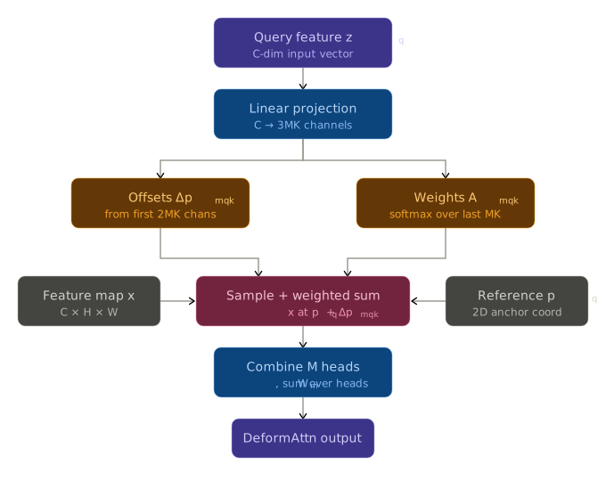
Both $\Delta p_{mqk}$ and $A_{mqk}$ branch from a single linear projection on $z_q$. No feature map keys are consulted.

No keys involved

Unlike Multi-Head Attention, the weights are not computed from a query-key dot product. The query alone decides where to look and how much to weight each location. This is the defining departure from standard attention.

Sparse in count, not in reach

The constraint is on how many locations are sampled (K=4 per head), not how far the offsets can reach — $\Delta p_{mqk}$ is unconstrained in range. This is the key distinction from local-window attention (e.g. Swin Transformer) or CNNs, which restrict the radius. DeformAttn restricts the budget.

The sample locations $p_q+\Delta p_{mqk}$ are generally fractional coordinates, so the feature map is read via bilinear interpolation — same mechanism as Deformable Convolution.

Multi-scale extension

$$\text{MSDeformAttn}(z_q,{\hat{p}}_q,x^l)=\sum _{m=1}^M{W}_m\left[\sum _{l=1}^L\sum _{k=1}^K{A}_{mlqk}\cdot W_m^{\prime }\cdot x^l({\varphi }_l({\hat{p}}_q)+\Delta p_{mlqk})\right]$$

Changes from single-scale: $L$ feature levels, a normalized reference point rescaled per level by ${\varphi }_l$, and each head now sampling $LK$ locations with one softmax across all of them.

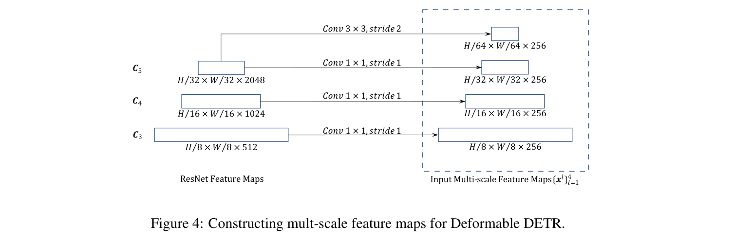
Building the pyramid (A.2)

No FPN. C3–C5 each go through a $1\times 1$ conv to $C=256$, plus a fourth level ($L=4$) from a $3\times 3$ stride-2 conv on C5 (stride 64). The “multi-scale input” is just four channel-aligned projections of backbone stages:

Why the normalized reference point is the glue

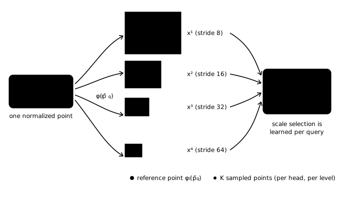
A single query must address four feature maps of different resolutions with one coordinate — that’s the whole reason ${\hat{p}}_q$ lives in $[0,1{]}^2$ and ${\varphi }_l$ just unnormalizes it per level. Each head then predicts a separate set of $K$ offsets per level (in that level’s pixel units), and one softmax spans all $L\times K$ weights:

The cross-level softmax is the FPN replacement

Because the softmax spans levels, scale selection is soft and learned per query — a small-object query can put nearly all its weight on the stride-8 level. Cross-scale routing lives in the attention weights, not in a fixed top-down pathway. Ablation: adding FPN on top gives nothing.

The token view (encoder)

The encoder input is literally the flattened pixels of all four levels concatenated into one sequence (~20k+ tokens — this is why linear complexity mattered). No patchification; the tokens are the conv feature vectors. Each pixel-token is its own query, with its own location as reference point, and gets two positional signals:

1. a fixed sinusoidal 2D encoding of its normalized location, and
2. a learned scale-level embedding $e_l$ (same vector for every token of level $l$).

Both are needed because the normalized coordinate is scale-blind: pixel $(0.5,0.5)$ at stride 8 and stride 32 would otherwise be positionally identical. And since DeformAttn has no query–key dot product, positional embeddings act only through the query side — they shape which offsets/weights a query predicts, never any key matching.

In the decoder, only cross-attention uses MSDeformAttn (queries → encoder tokens); self-attention among the $N$ object queries stays standard (cost is small).

Decoder object queries and the reference point

In DETR, the $N$ object queries carry no spatial information — specialization emerges implicitly through bipartite matching over hundreds of epochs. Deformable DETR keeps the same idea — learned, image-independent priors — but makes the spatial part explicit: the reference point ${\hat{p}}_q=\sigma (W{z}_q)$ is a deterministic function of the fixed query embedding, so after training each query has a fixed anchor point, identical for every image. The $N=300$ queries are effectively 300 learned anchor locations (later work — Anchor DETR, DAB-DETR — just parameterizes queries as anchors directly).

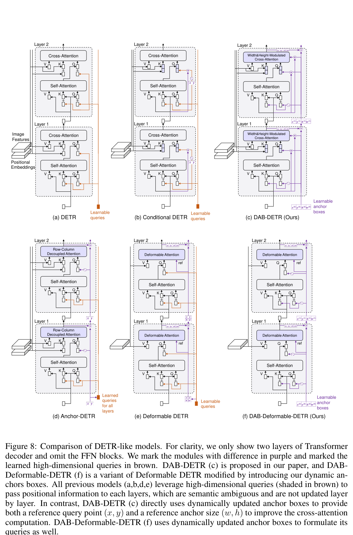
Where this sits in the DETR family — see DAB-DETR Fig. 8

DAB-DETR’s comparison figure lines up all six variants. Panel (e) is Deformable DETR — note it already carries an explicit reference point (ref, in orange) into deformable cross-attention but still passes a high-dimensional learned query for content. Panel (f), DAB-Deformable-DETR, keeps the deformable sampling untouched and only swaps that query for a dynamic 4D anchor box (in purple), feeding both a reference point and a reference size $(w,h)$ — the two mechanisms are orthogonal, which is why they compose in ~10 lines of code.

Boxes are residuals on the reference point (A.3)

The detection head does not predict absolute coordinates. The box center is a residual in inverse-sigmoid space:

${\hat{b}}_q=\{\sigma (b_{qx}+{\sigma }^{-1}({\hat{p}}_{qx})),\sigma (b_{qy}+{\sigma }^{-1}({\hat{p}}_{qy})),\sigma (b_{qw}),\sigma (b_{qh})\}$

The reference point is literally the initial guess of the box center — the same point the query attends around is the point its box is anchored to, so “where I look” and “what I predict” are spatially locked together. The paper credits this correlation for faster convergence. (The linear layers predicting reference points and offsets train at 0.1× the base LR.)

Multiple objects at one location?

Nothing hard-assigns a query to a region: the box residual and sampling offsets are unconstrained, so a query can drift far from its anchor. De-duplication is DETR’s original mechanism — decoder self-attention (kept standard for exactly this) plus Hungarian matching pushing colliding queries onto different targets. No NMS anywhere.

Two-stage: an encoder-only detector proposes the queries

Motivation: one-stage anchors are content-blind — predicted from embeddings that have seen no image, they can only be well-spread priors. Two-stage lets the encoder propose them, RPN-style but end-to-end:

• Stage 1 = dense per-pixel detection on the encoder output. A detection head (3-layer FFN box regressor + binary foreground classifier) is applied to every encoder token — output is $\text{batch}\times {\sum }_l{H}_l{W}_l$ boxes, each anchored at its own pixel with a level-dependent base scale $s=0.05\cdot 2^{l-1}$ (the FPN-detector “level implies size” convention, smuggled back in). Trained with the same Hungarian loss, directly on the encoder — no decoder involved.
• Why not just make every pixel a decoder query? Decoder self-attention is quadratic in query count; tens of thousands of pixel-queries are infeasible. Hence: dense proposals → top-300 by score (no NMS — redundant proposals are deliberately let through for the decoder to sort out).
• Stage 2 initialization: the proposal box becomes the initial box for iterative refinement, and the query’s positional embedding is set to the positional encoding of the proposal coordinates — both anchor and query content derive from the encoder.

Variant	Reference point source	Query $z_q$ source
DETR	none — fully implicit	learned embedding
Deformable DETR (1-stage)	$\sigma (W{z}_q)$ — fixed per query	learned embedding
Deformable DETR (2-stage)	encoder proposal center	pos-enc of proposal coords

The progression

DETR trusts queries to figure out space implicitly. One-stage gives them an explicit anchor. Two-stage doesn’t trust the queries at all — the “elegant slot” idea is quietly retired. Gains are additive (Table 1): 43.8 → 45.4 (+refinement) → 46.2 AP (+two-stage), concentrated in small objects.

Iterative bounding box refinement (§4.2)

Each of the $D=6$ decoder layers refines the box from the previous layer rather than predicting independently. The reference point for layer $d$ is the box center predicted by layer $d-1$, and sampling offsets are modulated by that box’s predicted width/height — so the attention window shrinks as the box tightens. Detection heads are not shared across layers. Gradients are blocked through the inverse-sigmoid of the previous box (RAFT-style detach, for stability), and offset-prediction biases are initialized at $\frac{1}{2K}$ scale so initial samples fall inside the previous layer’s box. See A.4 for the full formula.

Relation to deformable convolution

Setting $L=1$, $K=1$, $W_m^{\prime }=I$ recovers deformable convolution exactly. The lineage is Deformable Convolution → DeformAttn — not MHA with deformable sampling bolted on.

When does DeformAttn apply?

DeformAttn is a spatial-domain trick. It has three implicit assumptions that all depend on the feature map being a spatially coherent conv grid:

1. Reference points are meaningful 2D coordinates in a continuous space.
2. Offsets $\Delta p_{mqk}$ can point anywhere in that space with real-valued precision.
3. Bilinear interpolation can retrieve features at fractional coordinates.

This is why it works when you combine attention with CNNs (conv feature maps are dense, spatially coherent, and continuously interpolable) and why it doesn’t directly translate to a ViT — a ViT token at position $(3,5)$ has no neighbor at $(3.7,5.2)$; there is nothing to interpolate between.

The paper’s 2020 publication date matters here: this is still the CNN+attention hybrid era. The implicit assumption that you have a real spatial feature map is never stated because it was universal.

Rule of thumb

Use DeformAttn when (a) your keys live in a spatially structured feature map, and (b) you know the relevant information is spatially local to the query but don’t know exactly where. If the feature map has no spatial meaning (flat ViT tokens, language sequences), the offset mechanism loses its grounding.