Attention is all you need

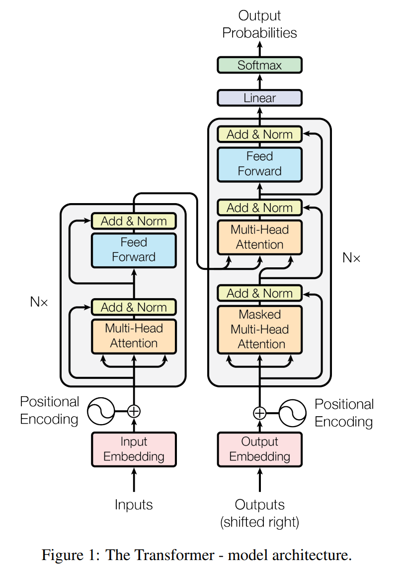
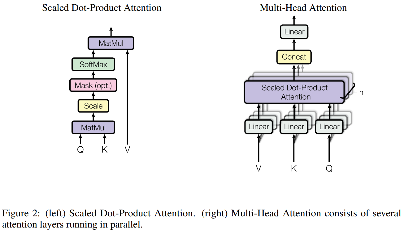
To really understand what’s going on, see Andrej’s Neural Networks: Zero to Hero lecture. Specifically, Lecture 7: Lecture 7: Let’s build GPT: from scratch, in code, spelled out. Obviously GPT-2 is basically this, but using a lot of data.

Input, output and loss

Suppose we use the very basic character tokenizer, that maps every letter / symbol into some int.

batch_size = 4 # how many independent sequences will we process in parallel? B
block_size = 8 # what is the maximum context length for predictions? T

Then the x and y (batched) would both have shape of (B, T), like this:

inputs:
torch.Size([4, 8])
tensor([[24, 43, 58,  5, 57,  1, 46, 43],
        [44, 53, 56,  1, 58, 46, 39, 58],
        [52, 58,  1, 58, 46, 39, 58,  1],
        [25, 17, 27, 10,  0, 21,  1, 54]])
targets:
torch.Size([4, 8])
tensor([[43, 58,  5, 57,  1, 46, 43, 39],
        [53, 56,  1, 58, 46, 39, 58,  1],
        [58,  1, 58, 46, 39, 58,  1, 46],
        [17, 27, 10,  0, 21,  1, 54, 39]])

Targets is basically input, shifted by one. In each of this samples there are actually T samples for each “item”:

when input is [24] the target: 43
when input is [24, 43] the target: 58 
when input is [24, 43, 58] the target: 5 
when input is [24, 43, 58, 5] the target: 57

This is enforced by the loss function:

logits = logits.view(B*T, C)
targets = targets.view(B*T)
# For each batch and time, there's a corresponding expected output.
# There's mechanism in decoder-only self attention to make sure output for [24] only look at [24].
loss = F.cross_entropy(logits, targets)

Generation

One important aspect of transformer is that its parameter does not depend on T (context length). So you can start from one char, and then keep appending new result to the input and ask the network what’s the output. For a t size sequence, network also output t size output, we only need the last one here.

def generate(self, idx, max_new_tokens):
	# idx is (B, T) array of indices in the current context
	for _ in range(max_new_tokens):
	# crop idx to the last block_size tokens
	idx_cond = idx[:, -block_size:]
	# get the predictions
	logits, loss = self(idx_cond)
	# focus only on the last time step
	logits = logits[:, -1, :] # becomes (B, C)
	# apply softmax to get probabilities
	probs = F.softmax(logits, dim=-1) # (B, C)
	# sample from the distribution
	idx_next = torch.multinomial(probs, num_samples=1) # (B, 1)
	# append sampled index to the running sequence
	idx = torch.cat((idx, idx_next), dim=1) # (B, T+1)
	return idx

Building self attention

Let’s pay attention (pun not intended) for the very basic formula:

Attention (Q, K, V) = softmax (\frac{Q K ^{T}}{d _{k}}) V

Think about the following questions:

What’s softmax doing here?
What if we want each token to only attend to stuff before it? (This paper is machine translation so it does not matter)
What about that $d_{k}$ ?

Andrej’s interpretation:

Matrix multiplication is weight aggregation.

# toy example illustrating how matrix multiplication can be used for a "weighted aggregation"
torch.manual_seed(42)
a = torch.tril(torch.ones(3, 3))
a = a / torch.sum(a, 1, keepdim=True)
b = torch.randint(0,10,(3,2)).float()
c = a @ b

a= tensor([[1.0000, 0.0000, 0.0000],
		 . [0.5000, 0.5000, 0.0000],
           [0.3333, 0.3333, 0.3333]])
--
b= tensor([[2., 7.],
           [6., 4.],
           [6., 5.]])
--
c= tensor([[2.0000, 7.0000], 
		   [4.0000, 5.5000], 
		   [4.6667, 5.3333]])

Here this c is “mean of the first n tokens.” Assuming the b is of size TxC, we are basically computing for all context lengths. Using softmax there is just convenient way of creating weights between $[0, 1]$ to do this aggregation. Self attention make this weight learnable.

# version 4: self-attention!
torch.manual_seed(1337)
B,T,C = 4,8,32 # batch, time, channels
x = torch.randn(B,T,C)
 
# let's see a single Head perform self-attention
head_size = 16
key = nn.Linear(C, head_size, bias=False)
query = nn.Linear(C, head_size, bias=False)
value = nn.Linear(C, head_size, bias=False)
k = key(x)   # (B, T, 16)
q = query(x) # (B, T, 16)
wei =  q @ k.transpose(-2, -1) # (B, T, 16) @ (B, 16, T) ---> (B, T, T)
 
tril = torch.tril(torch.ones(T, T))
#wei = torch.zeros((T,T))
wei = wei.masked_fill(tril == 0, float('-inf'))
wei = F.softmax(wei, dim=-1)
 
v = value(x)
out = wei @ v
#out = wei @ x

For that scaled $d_{k}$ part, since we’re doing q@k there, if the inputs are all unit gaussian, wei’s distribution would be $head_size^{2}$ , thus making the softmax too sharp, converge to max.

Why Both Q and K?

The goal of q @ k.T is to produce a (B, T, T) weight matrix encoding how much each token attends to every other. You could ask: why two projections? Why not just q @ q.T?

The answer is asymmetry. q @ q.T forces the weight matrix to be symmetric — token $i$ ‘s affinity toward $j$ equals $j$ ‘s toward $i$ . But attention isn’t symmetric: “it” attending to “cat” doesn’t mean “cat” should attend to “it.” Separate Q and K projections let the matrix be asymmetric: Q encodes “what am I looking for?” and K encodes “what do I advertise about myself?” — genuinely different roles.

The factorization also has practical virtues: it’s data-dependent (weights are recomputed fresh per input, not fixed parameters) and low-rank ( $O (T \cdot d_{k})$ parameters vs. a raw $O (T^{2})$ weight matrix that wouldn’t generalize across positions).

So Q/K together give you an asymmetric, data-dependent, low-rank factorization of the attention weight matrix — each property doing real work.

The naming is borrowed from a key-value store analogy. Token $i$ ‘s query $q_{i}$ is “what am I looking for?”, token $j$ ‘s key $k_{j}$ is “what do I advertise?”, and $v_{j}$ is the actual content retrieved. The asymmetry is semantic, not mathematical — if you swapped $W_{Q} \leftrightarrow W_{K}$ you’d get the transpose of the weight matrix. The learned weights shape Q-space and K-space so that meaningful pairs have high dot product.

Single Head = One Scalar Per Token Pair

Each row $i$ of $Q K^{⊤} \in R^{T \times T}$ is $q_{i} K^{⊤}$ — token $i$ scoring every other token simultaneously. After softmax, row $i$ sums to 1: it’s a single probability distribution over positions. This means token $i$ must express all its attention needs — syntactic, semantic, positional — in one weighted average of $V$ . Softmax kills superposition: you can’t attend 70% to position 3 and 70% to position 7 at the same time within one head.

Multi-head attention escapes this by running $h$ independent heads, each with its own $W_{Q}^{h}, W_{K}^{h}, W_{V}^{h}$ projecting into a $d_{k} = d_{m o d e l} / h$ subspace. Two things happen at once:

Complexity is preserved — total FLOPs across all heads ≈ one full-dim head.

Each head gets its own distribution — head 1 might track syntax, head 2 coreference, head 3 local context. $W_{O}$ then mixes the concatenated outputs.

So multi-head isn’t just a chunked single lens — it’s parallel diverse lenses, each freed from the softmax-superposition constraint.

Multi-head attention

class MultiHeadAttention(nn.Module):
    """ multiple heads of self-attention in parallel """
 
    def __init__(self, num_heads, head_size):
        super().__init__()
        self.heads = nn.ModuleList([Head(head_size) for _ in range(num_heads)])
        self.proj = nn.Linear(n_embd, n_embd)
        self.dropout = nn.Dropout(dropout)
 
    def forward(self, x):
        out = torch.cat([h(x) for h in self.heads], dim=-1)
        out = self.dropout(self.proj(out))
        return out

Don’t forget linear layers

See that feed forward part in the diagrams? They are needed. Attention focus on “getting info from other times”, or communication. Feed forward layers mixes up the C channel, or think.

More tricks

To make the network able to handle large amount of data, we need regularization, which is done by
- LayerNorm, which is basically does norm in “input params” instead of in batch. So it doesn’t need to distinguish train / eval as there’s no running mean.
- Skip connection.
- Add dropout

Encoder / decoder / only

The left part of the diagram is encoder, the other is decoder. If you operate on the same domain for input and output, you can do decoder only.

My original notes for the paper

The use of self attention inside both encoder and decoder itself, not only encoder-decoder level “normal” attention
The clever positional encoding with sin and cos waves, and use residual blocks to propagate that information. You can think of it as a more concise way of binary encoding (for floats).

Transformer Architecture: The Positional Encoding

Multi-head attention is kinda like general attention where a linear layer is used when combining key and query, but probably better, as we could have multiple key, value, query now.

The OG transformer uses Absolute position embedding.

My code

def scaled_dot_product_attention(
    Q: Float[Tensor, " ... queries d_k"],
    K: Float[Tensor, " ... keys d_k"],
    V: Float[Tensor, " ... values d_v"],
    mask: Bool[Tensor, " ... queries keys"] | None = None,
) -> Float[Tensor, "... values d_v"]:
    # Q and K compose together to form the actual big softmax weighting tensor
    pre_softmax: Float[Tensor, "... queries keys"] = einx.dot(
        "... queries d_k, ... keys d_k -> ... queries keys", Q, K
    ) / math.sqrt(K.shape[-1])
    if mask is not None:
        pre_softmax = torch.where(mask, pre_softmax, -torch.inf)
    return softmax(pre_softmax, -1) @ V
 
class CausalMultiHeadAttention(nn.Module):
    def __init__(self, d_model: int, num_heads: int):
        super().__init__()
        assert not (d_model % num_heads)
        d_k = d_model // num_heads
        # We can combine them but that makes weight loading hard so I do the easy thing
        self.project_q = Linear(d_model, d_model)
        self.project_k = Linear(d_model, d_model)
        self.project_v = Linear(d_model, d_model)
        self.project_o = Linear(d_model, d_model)
        self.d_k = d_k
        self.num_heads = num_heads
 
    def forward(self, x: Float[Tensor, "... seq_len d_model"]) -> Float[Tensor, "... seq_len d_model"]:
        Q = self.project_q(x)
        K = self.project_k(x)
        V = self.project_v(x)
        Q = einx.rearrange("... seq_len (h d_k) -> ... h seq_len d_k", Q, h=self.num_heads)
        K = einx.rearrange("... seq_len (h d_k) -> ... h seq_len d_k", K, h=self.num_heads)
        V = einx.rearrange("... seq_len (h d_k) -> ... h seq_len d_k", V, h=self.num_heads)
        seq_len = x.shape[-2]
        before_output: Float[Tensor, "... h seq_len d_k_per_head"] = scaled_dot_product_attention(
            Q, K, V, mask=torch.tril(torch.ones((seq_len, seq_len)).bool())
        )
        before_output = einx.rearrange("... h seq_len d_k_per_head -> ... seq_len (h d_k_per_head)", before_output)
        return self.project_o(before_output)
 
class CausalMultiHeadAttentionWithRoPE(CausalMultiHeadAttention):
    def __init__(self, d_model: int, num_heads: int, max_seq_len: int, rope_theta: float):
        super().__init__(d_model, num_heads)
        self.rope = RoPE(theta=rope_theta, d_k=self.d_k, max_seq_len=max_seq_len)
 
    def forward(
        self,
        x: Float[Tensor, "... seq_len d_model"],
        token_positions: Integer[Tensor, " ... sequence_length"] | None = None,
    ) -> Float[Tensor, "... seq_len d_model"]:
        Q = self.project_q(x)
        K = self.project_k(x)
        V = self.project_v(x)
        Q = einx.rearrange("... seq_len (h d_k) -> ... h seq_len d_k", Q, h=self.num_heads)
        K = einx.rearrange("... seq_len (h d_k) -> ... h seq_len d_k", K, h=self.num_heads)
        V = einx.rearrange("... seq_len (h d_k) -> ... h seq_len d_k", V, h=self.num_heads)
        seq_len = x.shape[-2]
        if token_positions is None:
            token_positions = torch.arange(seq_len)
        Q = self.rope(Q, token_positions=token_positions)
        K = self.rope(K, token_positions=token_positions)
        before_output: Float[Tensor, "... h seq_len d_k_per_head"] = scaled_dot_product_attention(
            Q, K, V, mask=torch.tril(torch.ones((seq_len, seq_len), dtype=bool, device=x.device))
        )
        before_output = einx.rearrange("... h seq_len d_k_per_head -> ... seq_len (h d_k_per_head)", before_output)
        return self.project_o(before_output)
 
class TransformerBlock(nn.Module):
    def __init__(self, d_model: int, num_heads: int, d_ff: int, max_seq_len: int, rope_theta: float):
        super().__init__()
        self.norm_1 = RMSNorm(d_model)
        self.norm_2 = RMSNorm(d_model)
        self.mha = CausalMultiHeadAttentionWithRoPE(d_model, num_heads, max_seq_len, rope_theta)
        self.ff = SwiGLUFeedForward(d_model=d_model, d_ff=d_ff)
 
    def forward(self, x: Float[Tensor, "... seq_len d_model"]) -> Float[Tensor, "... seq_len d_model"]:
        x = self.mha(self.norm_1(x)) + x
        x = self.ff(self.norm_2(x)) + x
        return x
 
class TransformerLM(nn.Module):
    def __init__(
        self,
        d_model: int,
        num_heads: int,
        d_ff: int,
        context_length: int,
        rope_theta: float,
        vocab_size: int,
        num_layers: int,
    ):
        super().__init__()
        self.embedding = Embedding(num_embeddings=vocab_size, embedding_dim=d_model)
        self.transformers = nn.ModuleList(
            [TransformerBlock(d_model, num_heads, d_ff, context_length, rope_theta) for _ in range(num_layers)]
        )
        self.ln_final = RMSNorm(d_model)
        self.lm_head = Linear(d_model, vocab_size)
 
    def forward(self, x: Integer[Tensor, "... seq_len"]) -> Float[Tensor, "... seq_len token_size"]:
        x = self.embedding(x)
        for layer in self.transformers:
            x = layer(x)
        x = self.ln_final(x)
        x = self.lm_head(x)
        return x

Yanda's Random Notes

Explorer