Q-chunking

---

Notes written with Claude Code (Claude Opus 5.5) from a reading discussion.

---

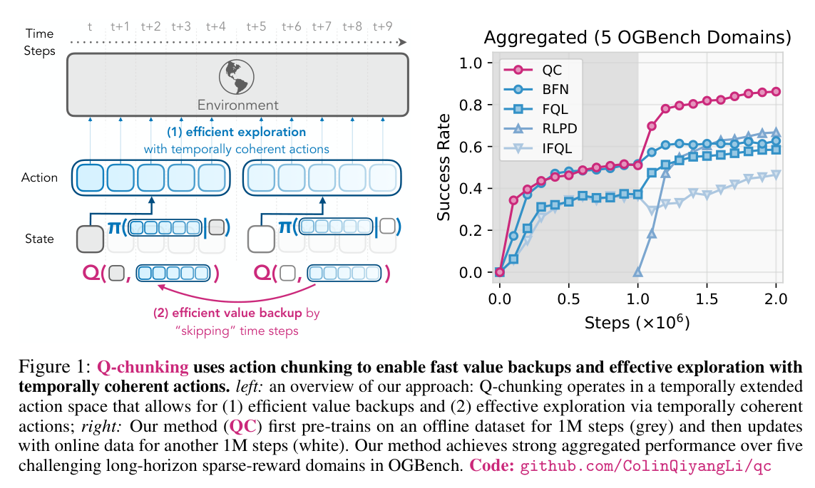
Offline-to-online RL on long-horizon, sparse-reward manipulation has two problems. Value propagates one step per backup, and exploration from a single-step policy is jittery and goes nowhere. The paper’s one idea: treat an $h$-step action chunk as a single macro-action and do ordinary RL over chunks. The policy outputs $a_{t:t+h}$ and executes it open-loop. The critic is $Q(s_t,a_t,\dots ,a_{t+h-1})$. Two things then come for free:

1. One-step TD in the chunk MDP is an $h$-step backup in the original MDP, without the off-policy bias of naive $n$-step returns.
2. A behavior constraint on chunks constrains short coherent behaviors from the data, not individually plausible actions. That gives structured exploration.

Concretely, for the main variant QC: from an offline dataset (later grown with online rollouts), train (a) a flow-matching BC model $f_{\xi }(A\mid s)$ over action chunks, and (b) a chunked critic $Q_{\theta }(s,A)$ with TD. To act, sample $N$ chunks from $f_{\xi }$, keep the one with the highest $Q$, and run its $h$ actions. There is no separate actor. The variant QC-FQL trains a one-step actor instead, so acting is a single forward pass.

Reading it backwards is probably closer to how it came about. Robot policies have predicted chunks since ACT. Given a model that outputs $h$ actions, the natural way to do RL with it is to make the chunk the unit of RL instead of un-chunking it. The macro-action view I had before reading the paper is the right mental model. The paper also quietly offers an answer to “why does chunking help robot policies”: the offline data is non-Markovian, and chunks capture that.

The recipe

Everything happens on chunks $A_t=a_{t:t+h}$. A training sample from the buffer is $(s_t,a_{t:t+h},r_{t:t+h},s_{t+h})$. The critic target is

$$Q_{\theta }(s_t,A_t)\leftarrow \sum _{k=0}^{h-1}{\gamma }^k{r}_{t+k}+{\gamma }^h{Q}_{\bar{\theta }}(s_{t+h},A_{t+h}^{\star })$$

where $A_{t+h}^{\star }$ comes from the same best-of-$N$ procedure used to act. QC’s whole loop, online phase (the offline phase is identical minus the environment):

\begin{algorithm}
\begin{algorithmic}
\REQUIRE flow BC policy $f_\xi(A \mid s)$, chunked critic $Q_\theta(s, A)$, dataset $\mathcal{D}$ (offline data)
\FOR{every environment step $t$}
    \IF{$t \bmod h = 0$}
        \STATE $A^1, \dots, A^N \sim f_\xi(\cdot \mid s_t)$
        \STATE $A^\star \gets \arg\max_i Q_\theta(s_t, A^i)$ \COMMENT{a new chunk only every $h$ steps}
    \ENDIF
    \STATE execute the next action of $A^\star$, observe $r_t, s_{t+1}$, add to $\mathcal{D}$
    \STATE update $f_\xi$ with the flow-matching loss on chunks from $\mathcal{D}$
    \STATE update $Q_\theta$ with the chunked TD loss, $A^\star_{t+h}$ from best-of-$N$
\ENDFOR
\end{algorithmic}
\end{algorithm}

Note what is not there: no policy-gradient step, no actor. The flow is pure BC (on a dataset that keeps growing online), and all the RL lives in $Q$ and in the argmax.

Why the chunked backup is unbiased when n-step isn’t

The paper’s equations put “biased” under the $n$-step reward sum and “unbiased” under the identical-looking chunked one. The difference is only what $Q$ is conditioned on.

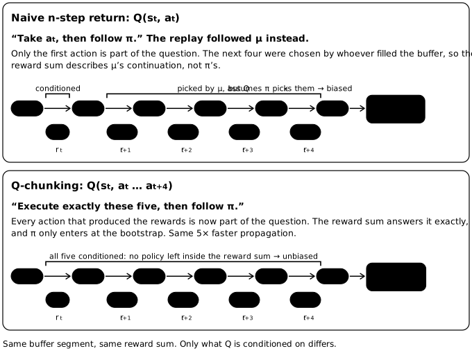
One-step off-policy TD is fine because a transition $(s,a,r,s^{\prime })$ is a sample of the environment’s response to $(s,a)$, no matter who chose $a$. Naive $n$-step breaks that: actions $a_{t+1},\dots ,a_{t+n-1}$ were chosen by the behavior policy, yet $Q^{\pi }(s_t,a_t)$ claims $\pi$ chose them. (The general argument is in Why one-step TD works off-policy.)

Q-chunking changes the question so that those actions are inputs. $Q(s_t,a_{t:t+h})$ asks “what if I execute exactly these $h$ actions, then follow $\pi$?“. The replayed rewards answer exactly that. At training time the chunk still comes from the replay buffer. It no longer matters who picked it, because every one of its actions is conditioned on.

It's not a clever n-step estimator

It’s plain one-step TD in an MDP whose action space is ${\mathcal{A}}^h$, with reward ${\sum }_k{\gamma }^k{r}_{t+k}$ and transition $s_t\to s_{t+h}$. The faster value propagation is a side effect of that MDP having $h$× fewer decision points.

The data isn’t Markov, but the environment is

The paper motivates the chunk-space behavior constraint with “offline data often exhibits non-Markovian structure”. At first that sounds like it undermines RL. It doesn’t, because two different things are being called Markov:

• The environment is a Markov MDP: $p(s_{t+1}\mid \text{history})=p(s_{t+1}\mid s_t,a_t)$. All the RL machinery needs only this.
• The behavior policy that produced the data need not be: a human or a scripted controller acts on intent, subtask, or a plan that isn’t in $s$.

Multimodality alone isn’t the issue; a stochastic Markov policy can be 50% left / 50% right. The issue is temporal correlation. A demonstrator who starts going left keeps going left, so the chunk distribution is roughly $\frac{1}{2}\text{LLLLL}+\frac{1}{2}\text{RRRRR}$. A single-step policy constrained to the per-step marginal can sample L, R, L, R, R, L, where every action looks fine on its own and the sequence is nothing the data ever did. A chunk policy matches the joint distribution, so it commits.

Is a chunk policy non-Markov? At primitive resolution, yes: $a_{t+1}$ depends on the chunk chosen at $t$, not only on $s_{t+1}$. At chunk resolution, $\pi (A_t\mid s_t)$ is perfectly Markov, and $P_h(s_{t+h}\mid s_t,A_t)$ is a valid induced transition. The Markov decision boundary moves from every step to every $h$ steps; nothing is broken.

So the constraint $D(\pi (A\mid s),{\pi }_{\beta }(A\mid s))\le \epsilon$ in chunk space says “stay among the short behaviors the data contains”: push in one direction, reach and close the gripper. Exploration then looks like skills instead of random dithering (the paper measures this: QC’s end-effector moves more per 5 steps and covers more states than the single-step BFN early in training). The paper frames this as the simplest hierarchical RL: the low-level skill is an open-loop action sequence, so the usual unstable bi-level optimization collapses into one RL problem.

Best-of-N is the policy, not a teacher

The behavior constraint for QC is implicit. Sampling $N$ chunks from $f_{\xi }$ and taking the argmax under $Q$ induces a distribution over executed chunks, and that distribution satisfies

$$D_{\mathrm{KL}}({\pi }_{\text{BoN}}\Vert f_{\xi })\le \log N-\frac{N-1}{N}$$

for any scorer. So there’s no actor that could drift outside the bound after training. Best-of-$N$ is the policy, used both to act and to produce $A_{t+h}^{\star }$ in the TD target. RL never changes the flow’s weights. It changes $Q$, which changes which proposals win. (Why the bound holds, and the family resemblance to AWR and CFGRL: Best-of-N sampling.)

• Proposal vs policy. $f_{\xi }$ is the proposal distribution: it suggests plausible robot motions; $Q$ chooses among them. Only at $N=1$ is the executed policy equal to $f_{\xi }$.
• $N$ is the constraint knob. Small $N$ means close to BC; large $N$ means more aggressive improvement and more exposure to $Q$‘s errors on rare samples.
• The reference moves. $f_{\xi }$ keeps training on the growing dataset online, so the constraint is always relative to the current data, not frozen to the offline prior.
• The cost is real: every chunk decision means $N$ flow samples (10 ODE steps each) plus $N$ critic calls, at inference too.

QC-FQL: put the improvement into the weights

QC-FQL is the answer to “why not just change the model weights?“. It’s FQL applied on ${\mathcal{A}}^h$ (FQL is exactly the $h=1$ case).

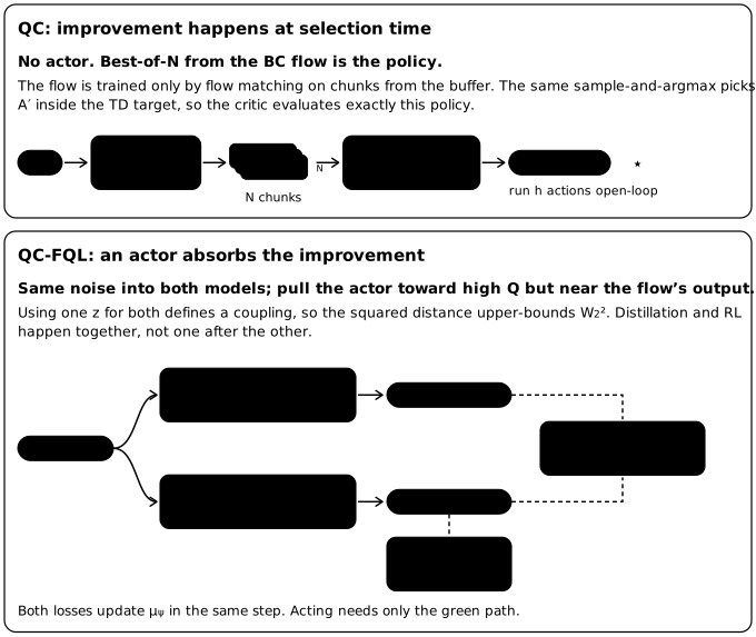
There are three networks: the flow BC model $f_{\xi }$ (same as QC), the chunked critic $Q_{\theta }$, and a one-step actor ${\mu }_{\psi }(s,z)$ that maps Gaussian noise to a full chunk in a single forward pass. “One-step” means one network evaluation instead of integrating the flow ODE, not one environment step. The actor loss is

$$\mathcal{L}(\psi )=\alpha \Vert {\mu }_{\psi }(s,z)-z^1(s,z){\Vert }_2^2-Q_{\theta }(s,{\mu }_{\psi }(s,z))$$

where $z^1$ is what the flow produces by integrating from the same noise $z$. So the "$\mu -f$" term is not a difference of network outputs ($f_{\xi }$ outputs a velocity). It is the L2 distance between the two final chunks generated from one $z$. Feeding both the same noise defines one particular coupling of the two distributions, and $W_2^2$ is the minimum over couplings, so this loss upper-bounds $\alpha W_2^2({\pi }_{\psi },f_{\xi })$. $\alpha$ trades fidelity to the data for $Q$ improvement.

Distillation and RL happen in the same update, not as “distill, then fine-tune”. That’s the contrast with Shortcut models: both replace a multi-step sampler with a one-step map, but a shortcut model wants student = teacher. Here the student is deliberately pulled off the teacher toward high $Q$. ${\mu }_{\psi }$ is better thought of as an amortized policy-improvement operator than as a distilled flow.

	where improvement happens	cost to act
QC	search: best-of-$N$ at every decision	$N$ flow samples + $N$ $Q$ calls
QC-FQL	inside ${\mu }_{\psi }$‘s weights, via $-Q$ + $W_2$ pull	one forward pass
CFGRL	inside the guided sampling dynamics	2× flow passes per step

FQL

FQL (Park et al., 2025) is the $h=1$ recipe above: a TD3+BC-style actor-critic whose BC term is distillation from a flow policy with shared noise. The paper doesn’t need anything more from it.

What the results lean on

Setup (snapshot)

• Tasks: 5 OGBench domains (scene, puzzle-3x3, cube-double/triple/quadruple; 5 tasks each), sparse reward, 1M–3M-transition play datasets (100M for cube-quadruple). Plus 3 robomimic tasks from multi-human data (300 trajectories each).
• Protocol: 1M offline gradient steps, then 1M online environment steps; same objective and same $N$/$\alpha$ in both phases.
• Networks: small MLPs (4×512), state-based, 10 flow steps. Not a pretrained VLA. $h=5$ by default, critic ensemble $K=2$.

• Chunking is what does the work. BFN (the same best-of-$N$ flow method on single actions) and BFN-n / FQL-n (single-action critics with $n$-step returns) are all clearly worse, most visibly on the hardest domains: after online training, QC reaches 64 / 73 on cube-triple / quadruple versus 41 / 36 for the best non-chunked baselines (RLPD, FQL-n).
• The expressive behavior model is required. Running chunked RL with an off-the-shelf Gaussian actor (RLPD-AC, even with a BC loss) mostly fails on the hard tasks. (Why a Gaussian is a poor behavior model yet a flow is hard to do RL on: RL with generative policies.)
• Chunk length is a real hyperparameter. For QC-FQL on cube-triple, $h=10$ is best, $h=25$ learns faster early but ends lower, and $h=50$ never succeeds: long open-loop chunks lose reactivity and are hard to predict. The authors leave choosing $h$ (or adaptive chunk boundaries) open.
• Open-loop chunks are a narrow slice of non-Markovian policies. Tasks that need tight feedback inside a chunk are a stated limitation.
• A larger critic ensemble ($K=10$) helps both QC and BFN a lot; a higher update-to-data ratio doesn’t help QC.