CFGRL

---

Notes written with OpenAI Codex (GPT-5) from a reading discussion.

---

Suppose we have an offline dataset and want a policy better than the behavior in that dataset. AWR would fit a new policy while giving high-advantage actions larger training weights. CFGRL instead turns “this action is good” into a condition of a generative policy. It trains one model to generate both ordinary dataset actions and actions under that condition, then contrasts the two distributions during sampling. The contrast is the improvement direction; a guidance weight $w$ controls how strongly it is followed.

The entire method is:

1. Give every dataset action an outcome condition. With a value function this can be the binary label $o=1[A(s,a)\ge 0]$; with goal-conditioned BC it is a future state that the trajectory actually reached.

2. Train one conditional flow policy on these examples. Randomly drop the condition on $10\%$ of examples, so the same network also learns unconditional BC.

3. At inference, query the network once without the condition and once with the desired condition. At every flow step use

   $$v_{\mathrm{guided}}=v_{\mathrm{uncond}}+w(v_{\mathrm{cond}}-v_{\mathrm{uncond}}).$$

   For the binary version, the desired condition is $o=1$; for GCBC, it is the goal $g$ we want to reach.

At $w=0$ this is ordinary BC. At $w=1$ it is ordinary conditional BC. At $w>1$ it pushes past the conditional policy toward actions that are especially characteristic of the desired outcome. Crucially, $w$ is chosen while sampling, so one trained model provides the whole sweep.

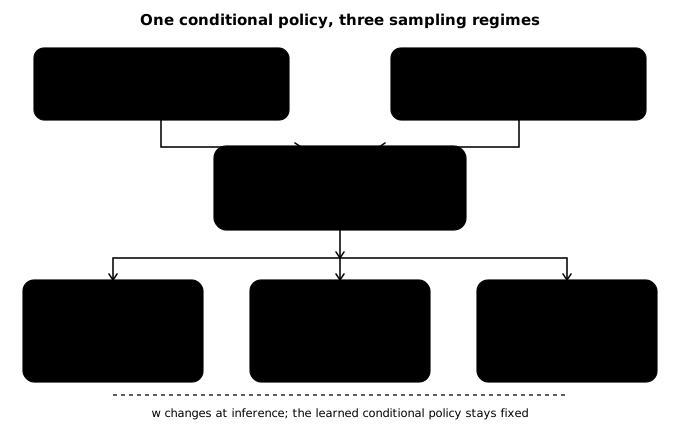
That is enough to implement CFGRL. Everything else follows from explaining why the conditional-unconditional contrast is a policy-improvement direction, and why goal-conditioned BC already contains the needed signal without an explicit value function.

Conditioning secretly multiplies BC by an outcome-likelihood factor

The central observation is just Bayes’ rule applied to how the training data were generated. Let $\hat{\pi }(a\mid s)$ denote the dataset’s behavior policy, and let $o$ be an outcome associated with the sampled action. Their joint distribution is

$$p(a,o\mid s)=\hat{\pi }(a\mid s)p(o\mid s,a).$$

If a conditional generative model perfectly learns the actions associated with outcome $o$, it learns

$$\begin{array}{rl}\hat{\pi }(a\mid s,o)& =\frac{\hat{\pi }(a\mid s)p(o\mid s,a)}{p(o\mid s)}\\ & \propto \hat{\pi }(a\mid s)p(o\mid s,a).\end{array}$$

This says something stronger than “conditioning filters the data.” The conditional policy is a product of:

• the behavior prior $\hat{\pi }(a\mid s)$, which keeps actions near the dataset; and
• the outcome likelihood $p(o\mid s,a)$, which favors actions associated with the requested outcome.

If the outcome is chosen so that

$$p(o\mid s,a)\propto f(A^{\hat{\pi }}(s,a))$$

for a nonnegative, nondecreasing function $f$, then conditioning has already constructed the policy

$${\pi }_1(a\mid s)\propto \hat{\pi }(a\mid s)f(A^{\hat{\pi }}(s,a)).$$

It remains close to actions the behavior could produce, but reallocates probability toward actions with higher advantage. The improvement proof follows directly. At each state,

$${\mathbb{E}}_{a\sim {\pi }_1}[A(a)]=\frac{{\mathbb{E}}_{a\sim \hat{\pi }}[A(a)f(A(a))]}{{\mathbb{E}}_{a\sim \hat{\pi }}[f(A(a))]}.$$

The reference policy has ${\mathbb{E}}_{\hat{\pi }}[A]=0$. Since $f(A)$ grows with $A$, the two quantities have nonnegative covariance, so the numerator is nonnegative. The conditioned policy therefore has nonnegative expected reference-policy advantage at every state, which is the standard condition for policy improvement.

This is the RL content of the method: choose a condition whose likelihood rises with advantage, and conditional density estimation becomes a regularized policy-improvement step.

Guidance exposes and amplifies the factor introduced by conditioning

Knowing that the conditional density is a useful product does not yet tell us how to sample from

$$\hat{\pi }(a\mid s)p(o\mid s,a{)}^w.$$

This is where the generative-model machinery enters. A diffusion or flow sampler moves an action through a learned vector field. Products are convenient because the log-density gradient of a product is a sum:

$${\nabla }_a\log \left[\hat{\pi }(a\mid s)p(o\mid s,a)\right]={\nabla }_a\log \hat{\pi }(a\mid s)+{\nabla }_a\log p(o\mid s,a).$$

Bayes’ rule gives the second term without training a separate outcome classifier:

$${\nabla }_a\log p(o\mid s,a)={\nabla }_a\log \hat{\pi }(a\mid s,o)-{\nabla }_a\log \hat{\pi }(a\mid s).$$

So the difference between the conditional and unconditional model fields isolates the direction contributed by the outcome likelihood. Multiplying that difference by $w$ gives

$$\begin{array}{rl}{s}_w& =s_{\mathrm{uncond}}+w(s_{\mathrm{cond}}-s_{\mathrm{uncond}})\\ & ={\nabla }_a\log \left[\hat{\pi }(a\mid s)p(o\mid s,a{)}^w\right].\end{array}$$

This is ordinary Classifier-free guidance, except the condition means “good action” or “reaches this goal” rather than “matches this text prompt.” Guidance is useful here not merely because it sharpens a condition, but because the condition was constructed to encode advantage. Turning up CFG therefore turns up a policy-improvement factor.

Why no explicit optimality classifier appears

One could train $p(o\mid s,a)$ directly and add its gradient to the behavior-policy field. That classifier would have to remain accurate on partially noised, potentially out-of-distribution actions; exploiting such a learned gradient is risky. Conditional and unconditional policy fields provide the same likelihood-ratio direction through Bayes’ rule, using only standard conditional generative-model training.

One network learns both ingredients before guidance is ever applied

The implementation uses Flow Matching. For each dataset action $a$, sample Gaussian noise $a_0$ and time $t$, interpolate

$$a_t=(1-t)a_0+ta,$$

and regress the velocity network toward the straight conditional velocity:

$${\Vert v_{\theta }(a_t,t,s,o)-(a-a_0)\Vert }^2.$$

There is no RL loss and no guidance weight in this objective. The outcome condition is replaced with $\varnothing$ on $10\%$ of examples, teaching the same parameters two distributions:

$$v_{\mathrm{uncond}}=v_{\theta }(a_t,t,s,\varnothing ),v_{\mathrm{cond}}=v_{\theta }(a_t,t,s,o).$$

Sampling starts from Gaussian action noise. At every integration step the model is queried twice, the two velocities are combined with the chosen $w$, and the action is advanced along the guided velocity. Training and sampling can be summarized as:

\begin{algorithm}
\begin{algorithmic}
\REQUIRE offline data $D$, an outcome-labeling rule, guidance strength $w$
\WHILE{training}
    \STATE Sample $(s,a)$ from $D$ and attach its outcome condition $o$.
    \STATE With probability $0.1$, replace $o$ with $\varnothing$.
    \STATE Sample $a_0$ from Gaussian noise and $t$ uniformly from $[0,1]$.
    \STATE Set $a_t \gets (1-t)a_0+ta$.
    \STATE Regress $v_\theta(a_t,t,s,o)$ toward $a-a_0$.
\ENDWHILE
\STATE At inference, initialize $a$ from Gaussian noise.
\WHILE{integrating the flow}
    \STATE $v_u \gets v_\theta(a,t,s,\varnothing)$
    \STATE $v_c \gets v_\theta(a,t,s,o_{\mathrm{desired}})$
    \STATE Advance $a$ using $v_u+w(v_c-v_u)$.
\ENDWHILE
\RETURN $a$
\end{algorithmic}
\end{algorithm}

The guidance identity above is exact for density scores, while the implementation predicts flow velocities. Prior work relates these parameterizations, and the same linear combination works empirically, but the exact score-space identity should be distinguished from this practical velocity-space transfer.

With a critic, “good” is just a label on every dataset action

In the ordinary offline-RL version, first learn $Q(s,a)$ and $V(s)$ with IQL, then compute

$$A(s,a)=Q(s,a)-V(s).$$

Each transition receives the binary label

$$o=1[A(s,a)\ge 0].$$

The flow policy is trained on every transition with an ordinary, equally weighted regression loss. The labels merely let it distinguish the distribution of nonnegative-advantage actions from the complete behavior distribution. During evaluation, asking for $o=1$ produces the conditional policy, and guidance beyond $w=1$ exaggerates the conditional-unconditional difference.

This explains both the similarity to and difference from advantage-weighted regression. AWR trains with

$${\mathbb{E}}_{(s,a)\sim D}\left[e^{A(s,a)/\beta }\log {\pi }_{\theta }(a\mid s)\right],$$

so high-advantage examples contribute larger gradients and the temperature is baked into the trained policy. CFGRL instead uses advantage to classify examples, keeps their training losses evenly weighted, and postpones the strength of reweighting until sampling. One trained network can therefore sweep $w$ without retraining.

The price is that CFGRL has not removed the RL problem: IQL still had to provide a trustworthy action ranking. CFGRL is the policy extraction step after value learning, not a replacement for learning values.

GCBC gets the same factor from trajectory structure instead of a critic

Goal-conditioned BC is the clever case because the dataset itself supplies an outcome label. Given a trajectory

$$s_0,a_0,s_1,a_1,\dots ,$$

sample a future offset

$$\Delta \sim \mathrm{Geom}(1-\gamma ),$$

take $g=s_{t+\Delta }$, and train

$$(s_t,g)\mapsto a_t.$$

This is hindsight relabeling, not a curriculum. The goal is a state the trajectory actually reached, not an intermediate waypoint invented by the learner. Each example says: “conditional on this rollout eventually reaching $g$, this was the action taken earlier at $s$.” At evaluation, $g$ is replaced by the goal we actually want.

Why sample the future offset geometrically? Because

$$P(\Delta =k)=(1-\gamma ){\gamma }^k,$$

so the probability of selecting $g$ as the hindsight future is proportional to its discounted visitation probability:

$$\begin{array}{rl}{p}^{\gamma }(g\mid s,a)& \propto \sum _{k\ge 0}{\gamma }^{k}P(s_{t+k}=g\mid s_t=s,a_t=a)\\ & =Q^{\hat{\pi }}(s,a,g)\end{array}$$

for the goal-reaching reward $r_g(s)=1[s=g]$.

Now apply the same Bayes argument as before. GCBC examples are produced by first choosing an action under the behavior policy and then sampling a future goal reached after that action:

$$p(a,g\mid s)=\hat{\pi }(a\mid s)p^{\gamma }(g\mid s,a).$$

Therefore the conditional policy learned by perfect supervised training is

$$\begin{array}{rl}{\pi }_{\mathrm{GCBC}}(a\mid s,g)& =\frac{\hat{\pi }(a\mid s)p^{\gamma }(g\mid s,a)}{p^{\gamma }(g\mid s)}\\ & \propto \hat{\pi }(a\mid s)Q^{\hat{\pi }}(s,a,g).\end{array}$$

GCBC has thus already performed one product-policy update with $f=Q^{\hat{\pi }}$. This $f$ satisfies the required monotonicity because, for fixed $s$ and $g$,

$$Q^{\hat{\pi }}(s,a,g)=A^{\hat{\pi }}(s,a,g)+V^{\hat{\pi }}(s,g),$$

and the second term does not depend on $a$.

GCBC is not estimating a queryable, calibrated $Q$-network. It directly learns the normalized product $\hat{\pi }Q$. But training the unconditional branch alongside it gives both

$$\hat{\pi }(a\mid s)\text{and}{\pi }_{\mathrm{GCBC}}(a\mid s,g)\propto \hat{\pi }(a\mid s)Q(s,a,g).$$

Their field difference isolates the direction contributed by the implicit goal-reaching value factor. Guidance simply turns that direction up:

$$\begin{array}{rcll}w=0& :& {\pi }_0=\hat{\pi },& \text{imitate the dataset},\\ w=1& :& {\pi }_1\propto \hat{\pi }Q,& \text{ordinary GCBC},\\ w>1& :& {\pi }_w\propto \hat{\pi }{Q}^w,& \text{CFGRL-guided GCBC}.\end{array}$$

This is why the goal-conditioned improvement is almost “free”: condition dropout already supplies unconditional BC, and the GCBC model already supplies the product with the implicit $Q$ factor. The only new operation is combining their two vector fields differently at inference.

The operator improves a fixed baseline once

CFGRL is mostly an offline/off-policy policy-extraction method, though the mathematical operator itself is not tied to offline data. Its required input is an action-dependent outcome signal whose likelihood rises with action quality:

• explicit advantage labels from a critic;
• a future goal that the action helped reach; or
• some other outcome condition with the same monotonic relationship.

Without such a signal, conditional and unconditional generation may still differ, but their difference has no reason to be an RL improvement direction.

The theory is anchored to one fixed reference policy $\hat{\pi }$ and its $A^{\hat{\pi }}$ or $Q^{\hat{\pi }}$. A genuine iterative algorithm would need to repeat

$${\pi }_k\stackrel{\text{evaluate}}{\to }{A}^{{\pi }_k}\stackrel{\text{relabel and train}}{\to }{\pi }_{k+1},$$

using a newly valid signal after every update. With fixed offline data, later policies may also favor actions the dataset scarcely covers. The paper avoids policy reevaluation, new data collection, and repeated distribution shift by applying the operator only once.

Large $w$ is not a substitute for these iterations. It keeps amplifying the same $A^{\hat{\pi }}$-derived direction; a second policy-improvement step would recompute the direction under the changed policy.

What is and is not guaranteed as $w$ increases

For every fixed $w\ge 0$, $f(A{)}^w$ is still nonnegative and nondecreasing, so the basic theorem establishes improvement over the original reference policy under its assumptions.

The paper additionally claims the stronger pairwise ordering $J({\pi }_{w_2})\ge J({\pi }_{w_1})$ for $w_2>w_1$. Its appendix rewrites ${\pi }_{w_2}$ as a reweighting of ${\pi }_{w_1}$ by a function of $A^{\hat{\pi }}$, then invokes a policy-improvement lemma that would require this factor to be monotone in $A^{{\pi }_{w_1}}$. That missing relationship is not established, and finite-MDP counterexamples exist. The safe interpretation is: $w$ controls how aggressively one fixed improvement factor is applied, but true return need not increase monotonically forever.

The experiments show a useful knob, not a universal RL solution

With explicit IQL advantages, CFGRL usually extracts a stronger policy than AWR across the ExORL and OGBench comparisons, while allowing the guidance sweep to happen without retraining. In the goal-conditioned experiments, $w=3$ improves over flow GCBC on most state and visual tasks, including pointmaze-giant ($4\to 30$ success) and visual-cube-single ($13\to 37$). Applying guidance at both levels of a hierarchical GCBC policy also produces large gains on several long-horizon tasks.

Some tasks are unchanged, remain at zero, or regress slightly. The useful range of $w$ ends when guidance pushes actions outside the region where the learned fields and optimality signal are reliable. Explicit CFGRL inherits critic errors; goal-conditioned CFGRL inherits the reachability and coverage of the behavior trajectories. The method also uses two network evaluations per flow step to obtain the conditional and unconditional fields.

The durable picture is therefore concrete: label actions by outcomes, train conditional and unconditional behavior in one generative policy, and use CFG to amplify the likelihood ratio between them. When that outcome likelihood increases with advantage, the familiar CFG direction becomes a policy-improvement direction. GCBC is the surprising special case where hindsight relabeling has already encoded the necessary value factor into the conditional action distribution.