Q learning

Recall dynamic programming algorithms Policy & value iteration

$$\begin{array}{rlrl}{v}_{k+1}(s)& =\mathbb{E}\left[R_{t+1}+\gamma v_k(S_{t+1})\mid S_t=s,A_t\sim \pi (S_t)\right]& & \text{(policy evaluation)}\\ v_{k+1}(s)& =\underset{a}{\max }\mathbb{E}\left[R_{t+1}+\gamma v_k(S_{t+1})\mid S_t=s,A_t=a\right]& & \text{(value iteration)}\\ q_{k+1}(s,a)& =\mathbb{E}\left[R_{t+1}+\gamma q_k(S_{t+1},A_{t+1})\mid S_t=s,A_t=a\right]& & \text{(policy evaluation)}\\ q_{k+1}(s,a)& =\mathbb{E}\left[R_{t+1}+\gamma \underset{a^{\prime }}{\max }{q}_k(S_{t+1},a^{\prime })\mid S_t=s,A_t=a\right]& & \text{(value iteration)}\end{array}$$

We have the analogous model -free TD algorithms:

$$\begin{array}{rl}{v}_{t+1}(S_t)& =v_t(S_t)+{\alpha }_t\left(R_{t+1}+\gamma v_t(S_{t+1})-v_t(S_t)\right)\text{(TD)}\\ q_{t+1}(s,a)& =q_t(S_t,A_t)+{\alpha }_t\left(R_{t+1}+\gamma q_t(S_{t+1},A_{t+1})-q_t(S_t,A_t)\right)\text{(SARSA)}\\ q_{t+1}(s,a)& =q_t(S_t,A_t)+{\alpha }_t\left(R_{t+1}+\gamma \underset{a^{\prime }}{\max }{q}_t(S_{t+1},a^{\prime })-q_t(S_t,A_t)\right)\text{(Q-learning)}\end{array}$$

Of course the value iteration on state $v$ cannot be sampled, so there’s no TD algorithm.

Q learning is an Off-Policy algorithm. It estimates the value of the greedy policy, whatever policy generated the data. (Why that is legitimate: Why one-step TD works off-policy.)

Acting greedy all the time would not explore sufficiently.

It’s soundness depend on a new theorem:

Q-learning control converges to the optimal action-value function, $q\to q^{\ast }$, as long as we take each action in each state infinitely often.

This is different from GLIE: the policy doesn’t need to converge to greedy. Works for any policy that eventually selects all actions sufficiently often (Requires appropriately decaying step sizes ${\sum }_t{\alpha }_t=\infty$, ${\sum }_t{\alpha }_t^2<\infty$, E.g., $\alpha =1/t^{\omega }$, with $\omega \in (0.5,1)$)

A comparison of SARSA and Q learning

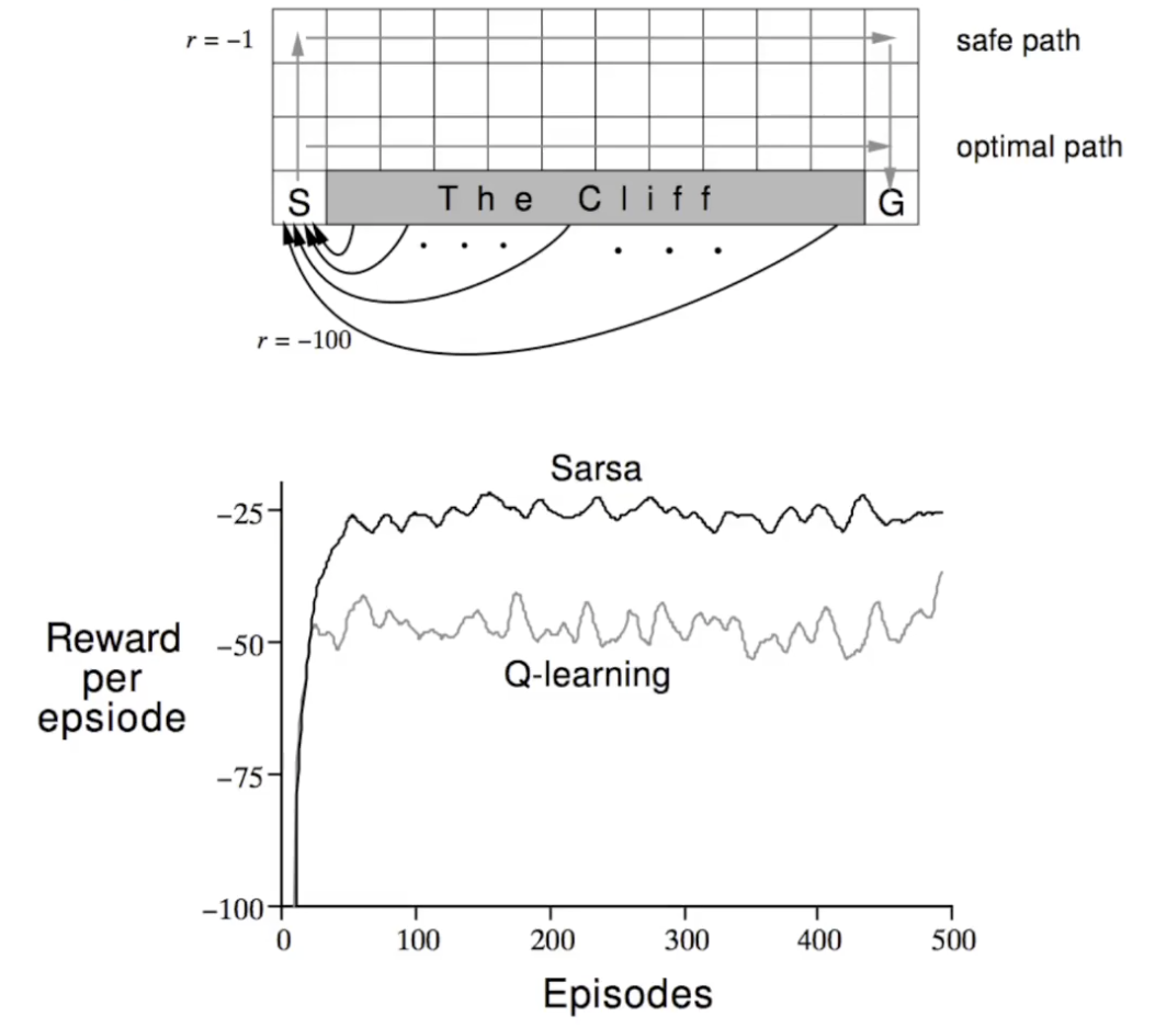In training time, SARSA gets higher reward since it learns that walking on the edge is dangerous, and it learns a safer path. Recall it’s using $ϵ$-greedy for both prediction and control. On the other hand, Q learning would stick to the optimal path, since according to its value estimation the optimal path is just the better one, since it has a larger $max$. So it would explore that path more often and got down more often. Note the final policy may be a more optimal one.

Overestimation

Recall

$$\underset{a}{\max }{q}_t(S_{t+1},a)=q_t(S_{t+1},\arg \underset{a}{\max }{q}_t(S_{t+1},a))$$

Uses same values to select and to evaluate. … but values are approximate

• more likely to select overestimated values
• less likely to select underestimated values

That “max” is persisting. Imagine you are in a state with 100 actions with stochastic outcome. If one of the action by chance got jackpot, then you would keep exploring that state. That leads to super slow convergence: blinded by overestimated values.

Another way to think about it: say we have two random variables: $X_1$ and $X_2$,

$$E[\max (X_1,X_2)]\ge \max (E[X_1],E[X_2])$$

our q estimation is a noisy estimation, and we are using the left one to estimate the right.

Double Q-learning

Store two action-value functions: $q$ and $q^{\prime }$

$$R_{t+1}+\gamma q_t^{\prime }(S_{t+1},\arg \underset{a}{\max }{q}_t(S_{t+1},a))\text{\hspace{1em}(1)}$$ $$R_{t+1}+\gamma q_t(S_{t+1},\arg \underset{a}{\max }{q}_t^{\prime }(S_{t+1},a))\text{\hspace{1em}(2)}$$

Each $t$, pick $q$ or $q^{\prime }$ (e.g., randomly) and update using (1) for $q$ or (2) for $q^{\prime }$.

This solves the issue because now the noise is decorrelated. The “max” when selecting the action may not actually leads to the “max” when actually getting the estimated Q value.

We can also extend this to SARSA.

Deep Q (DQN)

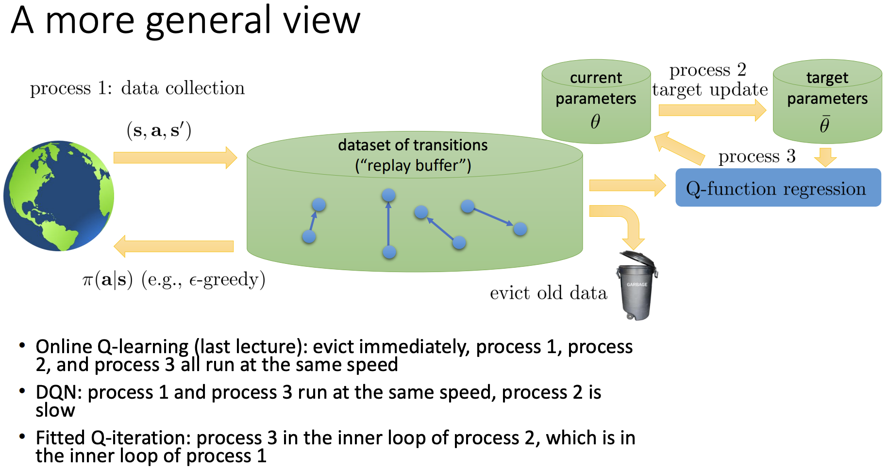
Use a NN as the function estimator for Q. The loss is TD loss. It comes from Fitted Q Iteration: we basically add a replay buffer and use transitions from the buffer instead of sampling with the policy.

$${\delta }_t=\stackrel{\text{TD Target}}{\overbrace{R_{t+1}+\gamma \underset{a}{\max }Q(S_{t+1},a)}}-\underset{\text{Former Q-value estimation}}{\underbrace{Q(S_t,A_t)}}\text{(TD Error)}$$

• A neural network: $O_t\mapsto {\mathbf{q}}_{\mathbf{w}}$ (action-out)
• An exploration policy: ${\pi }_t=ϵ\text{-greedy}({\mathbf{q}}_t)$, and then $A_t\sim {\pi }_t$
• A replay buffer to store and sample past transitions $(S_i,A_i,R_{i+1},S_{i+1})$
• Target network parameters ${\mathbf{w}}^{-}$, updated ${\mathbf{w}}^{-}\leftarrow \mathbf{w}$ occasionally (e.g., every 10000 steps)
• An optimizer to minimize the loss (e.g., SGD, RMSprop, or Adam)
• A Q-learning weight update on $\mathbf{w}$ (uses replay and target network):

$$\Delta \mathbf{w}=\left(R_{i+1}+\gamma \underset{a}{\max }{q}_{{\mathbf{w}}^{-}}(S_{i+1},a)-q_{\mathbf{w}}(S_i,A_i)\right){\nabla }_{\mathbf{w}}{q}_{\mathbf{w}}(S_i,A_i)$$

But wait, there’s still $\max$, so it can’t really handle continuous space well. It can handle complicated state space though.

\begin{algorithm}
\begin{algorithmic}
\STATE Initialize replay memory $D$ to capacity $N$
\STATE Initialize action-value function $Q$ with random weights $\theta$
\STATE Initialize target action-value function $\hat{Q}$ with weights $\theta^- = \theta$
\FOR{episode $= 1, \dots, M$}
    \STATE Initialize $s_1 = \{ x_1 \}$ and preprocessed $\phi_1 = \phi(s_1)$
    \FOR{$t = 1, \dots, T$}
        \STATE \COMMENT{Sampling}
        \STATE With probability $\varepsilon$ select a random action $a_t$, otherwise $a_t = \arg\max_a Q(\phi(s_t), a; \theta)$
        \STATE Execute $a_t$, observe reward $r_t$ and image $x_{t+1}$
        \STATE Set $s_{t+1} = s_t, a_t, x_{t+1}$ and preprocess $\phi_{t+1} = \phi(s_{t+1})$
        \STATE Store transition $(\phi_t, a_t, r_t, \phi_{t+1})$ in $D$
        \STATE \COMMENT{Training}
        \STATE Sample random minibatch of transitions $(\phi_j, a_j, r_j, \phi_{j+1})$ from $D$
        \IF{episode terminates at step $j+1$}
            \STATE $y_j \gets r_j$
        \ELSE
            \STATE $y_j \gets r_j + \gamma \max_{a'} \hat{Q}(\phi_{j+1}, a'; \theta^-)$
        \ENDIF
        \STATE Gradient descent step on $\big(y_j - Q(\phi_j, a_j; \theta)\big)^2$ w.r.t. $\theta$
        \STATE Every $C$ steps reset $\hat{Q} = Q$
    \ENDFOR
\ENDFOR
\end{algorithmic}
\end{algorithm}

Several ways to make training stable

Note the experience replay here. Since this is off policy, it can use previous samples to

• Reuse the interaction with the env.
• Avoid forgetting previous experiments and reduce the correlation between experiments

The latter $Q$ part in TD loss can be fixed (the target network), so it’s a fixed target, more like supervised learning.

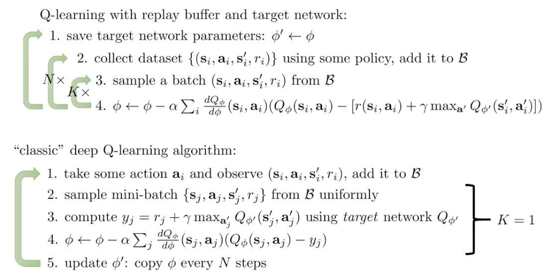
We can also avoid the sudden jump of “copy param every $N$” by using Polyak Averaging idea, linearly interpolating in parameter space:

$${\varphi }^{\prime }\leftarrow \tau {\varphi }^{\prime }+(1-\tau )\varphi$$

Double DQN is Double Q-learning with the target network playing the role of $q^{\prime }$, so no extra network is needed:

• standard: $y=r+\gamma Q_{{\varphi }^{\prime }}\left(s^{\prime },\arg {\max }_{a^{\prime }}{Q}_{{\varphi }^{\prime }}(s^{\prime },a^{\prime })\right)$
• double: $y=r+\gamma Q_{{\varphi }^{\prime }}\left(s^{\prime },\arg {\max }_{a^{\prime }}{Q}_{\varphi }(s^{\prime },a^{\prime })\right)$

Use the current network to select the action, the target network to evaluate it.

N step returns

See Multi-step returns. We can use n step return instead of single stage return:

$$y_{j,t}=\sum _{t^{\prime }=t}^{t+N-1}{\gamma }^{t^{\prime }-t}{r}_{j,t^{\prime }}+{\gamma }^N\underset{a_{j,t+N}}{\max }{Q}_{{\varphi }^{\prime }}\left(s_{j,t+N},a_{j,t+N}\right)$$

• Less biased target values when Q-values are inaccurate
• Typically faster training, especially early on: value propagates $N$ steps per backup instead of 1.
• Only actually correct when on-policy: the intermediate actions $a_{t+1},\dots ,a_{t+N-1}$ were picked by whoever filled the buffer, not by the policy we’re evaluating. See Why n-step returns break this.
• But we can ignore the problem and it seems to still be working well, or dynamically choose N to only on-policy data, or importance sampling. Or make $Q$ take all $N$ actions as input, which removes the bias entirely: Q-chunking.

Continuous Actions

There’s this ${\max }_{a}Q(s,a)$ here that’s hard to do for continuous actions.

Stochastic optimization

• We can random sample: sample a bunch in continuous space and pick the max we see. With a learned behavior policy as the sampler, this is Best-of-N sampling.
• Or use CEM or CMA-ES, doing Stochastic optimization to “guess the max” basically.

Use function class that’s easy to optimize

That’s based on the NAF paper, with Ilya Sutskever and Sergey Levine in the author list. The basic idea is to use a specific formula that can $max$ easily.

Use a NN to tell what’s the max

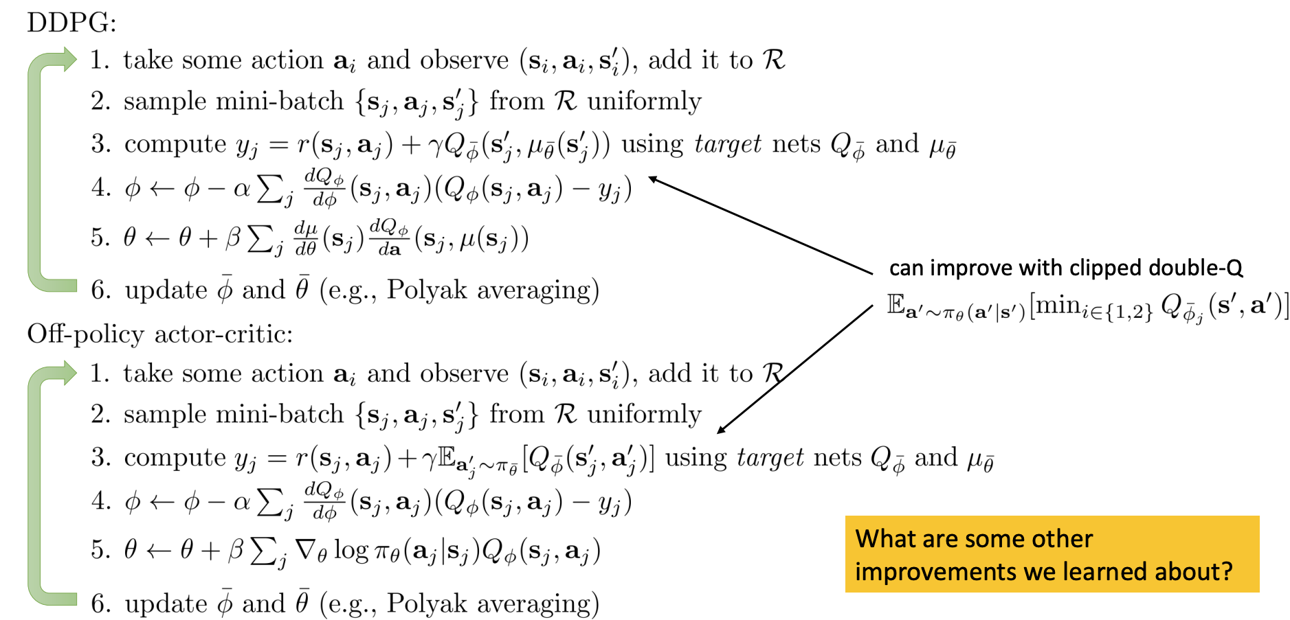
This is the DDPG idea: train another network ${\mu }_{\theta }(s)$ such that ${\mu }_{\theta }\approx \arg {\max }_a{Q}_{\varphi }(s,a)$. And we do not really train a new network. We just stitch them together, if the network outputs as we hope it outputs, the loss function would just optimize these two together.

You can argue this is quite similar to Actor-Critic

Practical tips

• Take times, may not stabilize easily
• Large replay buffers help stability
• Start with high exploration.
• Bellman error can be big. We can clip gradients or use Huber loss
• Double Q-learning help a lot, no downsides
• N-step return also help a lot, some downsides
• Needs tuning for exploration and learning rates
• Run multiple random seed, very inconsistent