Shortcut models

---

Notes written with OpenAI Codex (GPT-5.6 Sol Medium) from a reading discussion.

---

Flow Matching and diffusion models can generate good samples, but following their learned ODE usually costs dozens or hundreds of network evaluations. Simply reducing the number of Euler steps fails: the model predicts an instantaneous tangent, whereas a large jump must account for how that tangent will change as the trajectory curves.

Shortcut models solve this by conditioning one network on the desired step size $d$. At $d=0$ it behaves like an ordinary flow model. At larger $d$, it predicts the average velocity over an entire $d$-length transition, learned by matching two half-sized transitions. The cleanest lineage is binary progressive distillation, moved inside one jointly trained, step-conditioned network: no pretrained teacher, no sequence of student models, and the sampling budget can still be chosen at inference time.

Why flow matching cannot simply take larger steps

Optimal-transport flow matching constructs a straight conditional path for each independently sampled noise-data pair $(x_0,x_1)$:

$$x_t=(1-t)x_0+t{x}_1,v_t=x_1-x_0.$$

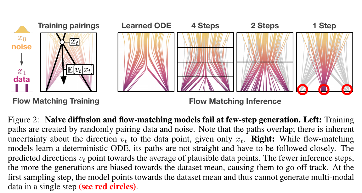
If both endpoints were known, the velocity would be constant and one step would reach $x_1$ exactly. The network does not know them, however; it receives only $(x_t,t)$ and therefore learns the conditional mean

$$\bar{v}(x,t)=\mathbb{E}[x_1-x_0\mid x_t=x].$$

That distinction is the source of nearly all the confusion here: the supervised conditional lines are straight, but the integral curves of the learned marginal field $\bar{v}$ generally are not. Intersecting conditional paths can imply different velocities at the same $(x,t)$; averaging them gives a deterministic field whose direction changes as the state moves.

The average is not a defective estimate of a sample’s destination. It is the correct local probability flux, satisfying the continuity equation

$${\partial }_t{p}_t(x)=-\nabla \cdot (p_t(x)\bar{v}(x,t)).$$

Once the identities of individual pairings are forgotten, their average velocity still moves the total density correctly. This is an infinitesimal statement—not permission to follow the current average all the way to $t=1$.

The two-mode example: why small steps preserve the information one step destroys

Let the data have two equally likely modes $z\in \{-2,+2\}$ and let the initial noise be $ϵ\sim \mathcal{N}(0,1)$. At $t=0$, $x_0=ϵ$. Evaluating the field at the particular location $x$ tells us that $ϵ=x$, while the independently paired destination is still unknown:

$$\begin{array}{rl}{u}_0(x)& =\mathbb{E}[z-ϵ\mid x_0=x]\\ & =\mathbb{E}[z]-x=-x.\end{array}$$

This is not the unconditional expectation $\mathbb{E}[z-ϵ]=0$. The field is pointwise: at $x=1.2$, the two possible velocities are $-3.2$ and $0.8$, whose average is $-1.2$.

A single Euler step of length one collapses every sample to the data mean:

$$x_1=x_0+u_0(x_0)=0.$$

A small step $h$, in contrast, moves only a fraction of the way:

$$x_h=x_0+h(-x_0)=(1-h)x_0.$$

At $h=0.01$, two noise samples retain $99\%$ of their separation. On the next query, their positions begin to reveal which mode is more plausible, so positive and negative trajectories bend toward $+2$ and $-2$. The model still averages at every step; the average is simply recomputed from an increasingly informative state.

The distinction worth keeping

A small Euler step uses the conditional mean as a local tangent. A one-step sampler treats that initial tangent as the whole trajectory. Averaging is not the failure; extrapolating the local average too far is.

The core idea: tell the model how far it must jump

The shortcut network receives the state $x_t$, time $t$, and requested step size $d$:

$$x_{t+d}^{\prime }=x_t+d{s}_{\theta }(x_t,t,d).$$

$s_{\theta }$ is normalized as a velocity, but its meaning depends on $d$:

• At $d=0$, it is the instantaneous flow $\bar{v}(x_t,t)$.
• At $d>0$, it is the average velocity of the complete finite transition from $t$ to $t+d$.

The second object accounts for how the local field would change along the way. It is not the $d=0$ prediction evaluated with a recklessly large Euler step.

At inference, choose a budget $M$, set $d=1/M$, and repeatedly apply

$$x\leftarrow x+d{s}_{\theta }(x,t,d),t\leftarrow t+d.$$

Thus the same model can make one whole-trajectory prediction, four quarter-trajectory predictions, or closely follow the flow with 128 steps.

Learning long shortcuts from two shorter ones

An exact ODE flow composes: going forward by $2d$ must equal going forward twice by $d$. With $x_{t+d}^{\prime }=x_t+ds(x_t,t,d)$, this gives the self-consistency target

$$s(x_t,t,2d)=\frac{1}{2}\left[s(x_t,t,d)+s(x_{t+d}^{\prime },t+d,d)\right].$$

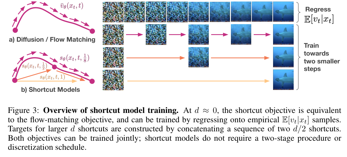
This is a genuine identity of the desired solution, not an arbitrary regularizer. Exact $d$ transitions would produce an exact $2d$ target, propagating inductively through $d,2d,4d,\dots$.

This is binary progressive distillation without the stages

Conventional progressive distillation begins with, say, a 128-step pretrained teacher. A student learns to replace every two teacher steps with one step, becoming a 64-step model. That student then becomes the teacher for a 32-step model, and the process repeats:

$$128\to 64\to 32\to 16\to 8\to 4\to 2\to 1.$$

It is binary because every phase doubles the step size. The normalized target for the student is the average of the two teacher velocities, exactly the form above.

Shortcut models perform this recursion jointly. One network represents every level via its $d$ input, and a slowly moving EMA copy supplies the smaller-step targets. This removes the pretrained teacher and phase schedule, while retaining the ability to sample at any trained budget.

Why the second state must come from the learned flow

End-to-end consistency training instead forms $(x_t,x_{t+d})$ by interpolating the same empirical noise-data pair at two noise levels. Given $x_t$, the paired data endpoint is hidden and ambiguous; different random pairings can provide incompatible later states for the same observed input. Regressing those targets introduces a compromise at every discretization interval.

Shortcut training constructs $x_{t+d}^{\prime }=x_t+ds(x_t,t,d)$ from the model’s deterministic marginal dynamics, then evaluates the second half-step there. The arbitrary empirical pairing appears only in the $d=0$ grounding loss, where its expectation is the correct local flux; it is not reintroduced into every finite-step target.

One network, two kinds of training examples

Equation 5 looks like two losses applied to the same example, but the implementation is easier to understand as two kinds of batch elements:

Branch	Model query	Target
Flow grounding	$s_{\theta }(x_t,t,0)$	Empirical velocity $x_1-x_0$
Shortcut bootstrap	$s_{\theta }(x_t,t,2d)$	Two EMA predictions of step size $d$

For a large-$d$ example, there is no flow-matching loss at that $d$, conditional or unconditional. Training it directly toward $x_1-x_0$ would recreate the original problem: that is the velocity of a randomly paired conditional line, not the integrated displacement of the deterministic marginal flow.

The paper uses about $75\%$ empirical targets and $25\%$ shortcut targets—roughly $16\%$ more compute than the base model. Shortcut sizes are discrete:

$$d\in \left\{\frac{1}{128},\frac{1}{64},\dots ,\frac{1}{2},1\right\},$$

plus the special $d=0$ branch. Training samples $t$ only from compatible multiples of $d$; accepting $d$ as input does not mean arbitrary continuous step sizes were demonstrated.

What prevents self-training from drifting

The TD-learning analogy is useful. The larger prediction is trained toward a target produced by the same function at smaller horizons, and stopgrad makes this a semi-gradient update. The difference is that there is no discount factor $\gamma <1$ making the composition operator a contraction. State error can instead be amplified by the flow Jacobian.

Three choices keep this workable:

1. EMA target weights ($\beta =0.999$) form a separate, slowly moving copy used for bootstrap targets and evaluation. They do not smooth or overwrite the online weights; this is a target network, separate from Adam’s moment estimates.
2. Weight decay stops the model from latching onto the nearly meaningless self-generated targets seen early in training.
3. Two-step bootstrap paths limit the error that can compound inside any one target.

What self-consistency does—and does not—guarantee

The composition equation is necessary for an exact flow, and the $d=0$ loss supplies a meaningful base case. But self-consistency alone has useless solutions such as $s=0$, and the paper does not prove uniqueness, stability, or convergence of the neural-network optimization. It is stronger than “this seems reasonable,” but weaker than TD policy evaluation with a contraction or a VAE objective with an ELBO.

Classifier-free guidance is baked into the shortcut hierarchy

CFG uses the same network with and without the class condition:

$$v_{\text{CFG}}(x,t\mid y)=v(x,t,\varnothing )+w[v(x,t,y)-v(x,t,\varnothing )].$$

There is no separate classifier: class dropout teaches the null-conditioned branch. ImageNet uses dropout $0.1$ and scale $w=1.5$. CFG combines local tangents, but applying the same interpolation to two long-range shortcut endpoints is generally different from integrating the guided field:

$$\mathrm{Flow}\left[v_u+w(v_c-v_u)\right]\ne \mathrm{Flow}[v_u]+w\left(\mathrm{Flow}[v_c]-\mathrm{Flow}[v_u]\right),$$

because the field is reevaluated all along the path. The authors therefore guide the base dynamics and let larger conditional shortcuts inherit that trajectory through self-consistency. A learned $d>0$ shortcut then needs one conditional forward pass; applying CFG again would double-count it.

The cost of baking guidance in

The CFG scale must be selected before training. A shortcut hierarchy trained around $w=1.5$ cannot safely be changed to $w=4$ at inference by applying ordinary CFG to its large displacements. Many-step sampling through the $d=0$ flow branch remains the exception: external local CFG is still appropriate there.

What the results establish—and what remains open

Under the controlled DiT-B comparison, shortcut models retain the base model’s many-step ability while degrading much more gracefully as the budget shrinks:

Dataset	128 steps	4 steps	1 step
CelebA-HQ, unconditional	6.9	13.8	20.5
ImageNet-256, class-conditioned	15.5	28.3	40.3

These are FID-50k scores; lower is better. The method beats the other end-to-end objectives in the table and is competitive with two-stage distillation. Progressive distillation reaches a better one-step ImageNet score in this comparison, but its final model gives up flexible many-step sampling and requires sequential training phases.

Few-step flow matching produces blur and mode collapse; shortcut errors are more often in fine details. The same noise can therefore produce a one-step preview and a more refined many-step version. Scaling also continues to help the bootstrapped model, and one-step shortcut policies retain much of the performance of iterative diffusion policies—useful evidence that the method is not tied to one image benchmark.

What the result still leans on

• One-step quality remains materially worse than many-step quality; the shortcut reduces the gap rather than eliminating it.
• Only the binary step hierarchy and compatible discrete time points are trained.
• Guidance is fixed during training.
• EMA and weight decay matter in practice, but their effects are not cleanly ablated.
• The central bootstrap procedure has no convergence or stability theorem.
• The noise-to-data mapping is still inherited from an expectation over random pairings. The authors identify changing that mapping—perhaps with a Reflow-like procedure—as an open direction.

The durable idea is not merely “condition on step size.” It is that ODE integration itself can be made a jointly learned, recursively compositional prediction problem: ground the infinitesimal behavior in data, teach each longer transition from two shorter ones, and expose the horizon to one shared model.