Pi 0.6

---

Notes written with Claude Opus 5.5 (Claude Code) from a reading discussion.

---

A VLA trained by imitation can only be as good as its demonstrations, and it never learns from the mistakes it makes once deployed. ${\pi }_{0.6}^{\ast }$ adds a way to learn from its own experience: autonomous runs, failures, slow successes, and human takeovers. The method, RECAP, turns RL into relabeling. A separate, smaller value model judges every sample in the data. Each judgment is binarized into one text token, Advantage: positive or Advantage: negative. The big VLA is then trained with its ordinary supervised losses while conditioned on that token. At deployment you simply prompt it with positive. No policy gradient ever touches the VLA, because all the RL judgment lives in the critic.

Operationally:

• Supervision: episodes with a human success/failure label, plus optional expert takeovers.
• Trained, in this order: a value model $V_{\varphi }(o,\ell )$, then a policy ${\pi }_{\theta }(a\mid o,\ell ,I)$ whose extra input $I$ is computed from $V$.
• Inference: set $I=$ positive and sample. Optionally, use CFG with $\beta >1$ to push harder.
• The one thing that differs from SFT: one extra conditioning token derived from the advantage.

In lineage terms this is CFGRL scaled to a flow-matching VLA (${\pi }_{0.6}$ is Pi 0.5 with a bigger backbone). The two changes are a task-specific threshold on what counts as “good” and human-gated DAgger corrections mixed into the data.

The recipe, in order: critic first, then actor

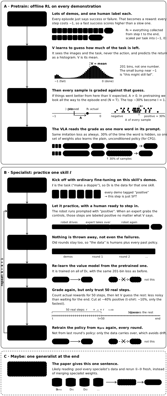
The whole method is three subroutines called on different data: collect, fit $V$, and fit $\pi$ using $V$. “The only thing that changes between steps is the data” means exactly that.

A. Pretraining is advantage-conditioned BC, and the paper calls it “offline RL”. The pretraining set $D_{\text{demo}}$ is tens of thousands of hours across many tasks and robots, and it includes failed episodes. The steps run in order: train $V_{\text{pre}}$ on all of it, use it to label every sample with $I_t$, then train ${\pi }_{\text{pre}}$. Mechanically, that last step is behavior cloning: the same π0.6 losses on the dataset’s actions, plus one extra input token. Nothing is reweighted and nothing is improved during training. The model just learns two things in one network: $\pi (a\mid o,\ell )$, “what the data did”, and $\pi (a\mid o,\ell ,I=1)$, “what the data did when it went better than expected”. The improvement happens only at inference, when you prompt with positive. The paper calls this offline RL because the label comes from a reward-trained critic, so the checkpoint contains a policy better than the data, even though training it was plain supervised learning. The ordering is strict. $V$ is fully trained first, then frozen and run on the fly inside the policy’s dataloader to produce $I_t$. “On the fly” means the labels aren’t precomputed. The two models are never trained jointly.

B. Specialists are where the robot practices. $D_{\ell }$ is lowercase ℓ, the task/language command. It is the dataset for one skill (espresso, box assembly, …), and it starts from that skill’s demos. The first specialist ${\pi }_{\ell }^0$ is plain SFT from ${\pi }_{\text{pre}}$ with $I=1$ on every demo. After that, each iteration runs the following steps:

1. Deploy the current specialist. Some runs are autonomous, and some have an expert who takes over when things go wrong.
2. Add every episode to $D_{\ell }$. Successes and failures both stay, and so does data from older iterations.
3. Refit $V_{\ell }^k$ and retrain ${\pi }_{\ell }^k$ on all of $D_{\ell }$. Both start from the pretrained checkpoints, not from iteration $k-1$.

The restart is deliberate because it reduces drift. Weights don’t accumulate, only data does. The paper ran 1–2 iterations per task.

C. The “final generalist” is one sentence in the paper. It says specialists are fine-tuned from the pretrained model “while the final generalist is trained from scratch.” That step isn’t in Algorithm 1. The natural reading is that specialists double as experience collectors. Their enriched $D_{\ell }$‘s get pooled with $D_{\text{demo}}$, and stage A is rerun fresh instead of merging specialist weights. “From scratch” most likely means “not continued from a specialist”, not “random init”, since everything starts from Gemma.

This is Algorithm 1 with the details from the appendix filled in:

\begin{algorithm}
\begin{algorithmic}
\REQUIRE multi-task demonstrations $D_{demo}$
\STATE Train $V_{pre}$ on $D_{demo}$ \COMMENT{binned Monte-Carlo returns}
\STATE Train $\pi_{pre}$ on $D_{demo}$, $I_t = 1[R_t - V_{pre}(o_t) > \epsilon_\ell]$ \COMMENT{about 30 percent positive}
\FOR{each target skill $\ell$}
    \STATE $D_\ell \gets$ demos for $\ell$
    \STATE $V^0_\ell \gets$ finetune $V_{pre}$ on $D_\ell$
    \STATE $\pi^0_\ell \gets$ finetune $\pi_{pre}$ on $D_\ell$ with $I = 1$ \COMMENT{plain SFT}
    \FOR{$k = 1$ to $K$}
        \STATE $D_\ell \gets D_\ell \cup$ rollouts of $\pi^{k-1}_\ell$ \COMMENT{takeover steps get $I = 1$}
        \STATE $V^k_\ell \gets$ finetune $V_{pre}$ on $D_\ell$
        \STATE relabel $D_\ell$ with 50-step advantages from $V^k_\ell$ \COMMENT{about 40 percent positive}
        \STATE $\pi^k_\ell \gets$ finetune $\pi_{pre}$ on $D_\ell$
    \ENDFOR
\ENDFOR
\end{algorithmic}
\end{algorithm}

Where the labels come from: a value model, not a Q-function

The reward is deliberately generic, because the only human input is one success label per episode. Each step costs $-1$, success ends at $0$, and failure ends with a large $-C_{\text{fail}}$. Values are normalized per task to $(-1,0)$ by maximum episode length. As a result, $V(o,\ell )$ reads as “minus the remaining time to success”, pushed far down when a failure is coming.

From $V$ the advantage is

$$A(o_t,a_t)\approx \sum _{t^{\prime }=t}^{t+N-1}{r}_{t^{\prime }}+V(o_{t+N})-V(o_t),$$

with $N=50$ in post-training. Pretraining uses $N=T$, so $A=R_t-V(o_t)$ and only one value call is needed per sample. That version is noisier, but it was fine at pretraining scale. In words, after the action that actually happened, did things go better than this state usually predicts? Nobody ever asks the critic “what if I had taken some other action $a$?” That would need a $Q(o,a)$ over a 50 Hz continuous action chunk, which is exactly what they avoid. They admit the cost: this is an on-policy Monte-Carlo estimate of the behavior policy, a mixture of humans and older policies. It measures “better than the data so far”, not “better than optimal”. It is less principled than an off-policy Q, but “simple and highly reliable.”

The 201-bin distribution is borrowed machinery, not their invention. The critic outputs a categorical distribution over 201 return bins, trained with cross-entropy on the bin of each sample’s realized return. The scalar is recovered as its expectation, $V={\sum }_b{p}_{\varphi }(b\mid o,\ell )v(b)$. This is C51-style distributional RL (Bellemare et al., 2017). The difference is that the targets are plain Monte-Carlo returns, not a distributional Bellman backup. A single trajectory contributes one bin per timestep, and the distribution emerges across many similar states. The paper doesn’t ablate bins against scalar regression. The usual reasons are that classification on bounded targets trains stably in big transformers, and that the distribution can keep “usually fast, sometimes catastrophic” bimodality instead of averaging it away. Their bounded $(-1,0)$ return makes binning natural.

Implementation snapshot (likely to date quickly)

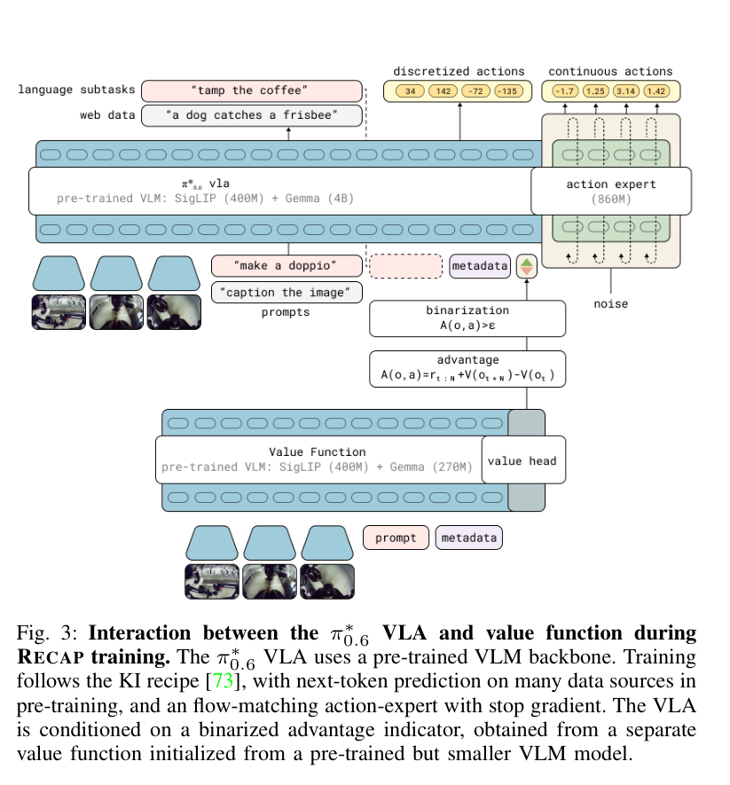
• VLA: ${\pi }_{0.6}$ with a Gemma 3 4B backbone and an 860M flow-matching action expert, trained with the Knowledge Insulating VLA recipe (FAST tokens plus a stop-gradient action expert). It outputs 50 Hz joint chunks and first predicts a text subtask $\hat{\ell }$ (Hi Robot-style).
• Value model: same design with a 670M Gemma 3 backbone, co-trained on some web VLM data to avoid overfitting. Because it’s small, running it on the fly during VLA training is cheap.
• Where the token goes: Advantage: positive/negative is placed after $\hat{\ell }$ and before the actions. Only the action likelihoods are affected, not subtask prediction.

How RECAP implements CFGRL

Recall CFGRL: the improved policy is the reference policy reweighted by “probability this action is an improvement”. Bayes turns that into a ratio of two policies, so no classifier is needed:

$$\hat{\pi }(a\mid o,\ell )\propto {\pi }_{\text{ref}}(a\mid o,\ell ){\left(\frac{{\pi }_{\text{ref}}(a\mid I,o,\ell )}{{\pi }_{\text{ref}}(a\mid o,\ell )}\right)}^{\beta }.$$

At $\beta =1$ this collapses to just sampling ${\pi }_{\text{ref}}(a\mid I,o,\ell )$. At $\beta >1$ it is Classifier-free guidance on the flow field. Either way, one network must represent both the conditional and the unconditional policy.

The CFG-style condition dropout is exactly what it looks like. RECAP drops $I$ from the input 30% of the time, the same trick as training a diffusion model without its prompt ~10% of the time. The written loss is $-\log \pi (a\mid o,\ell )-\alpha \log \pi (a\mid I,o,\ell )$. In practice, dropout sets the mix between the two terms and replaces $\alpha$. So the “mix conditional and unconditional” intuition from CFG is correct and still present.

What’s new is where the sharpening happens. CFGRL labels $I=1[A>0]$ and turns up $\beta$ at test time. RECAP uses $I=1[A>{ϵ}_{\ell }]$ with a task-specific threshold and usually stops at $\beta =1$.

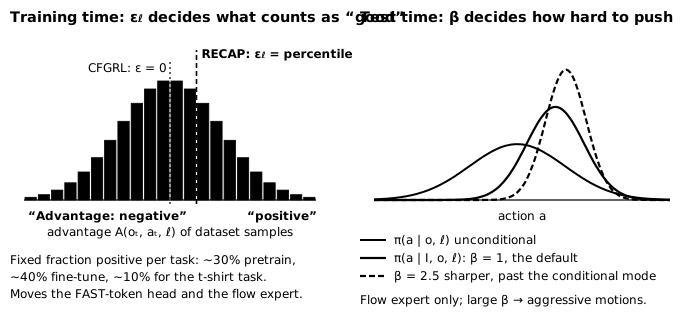
Both knobs make the “good” distribution more selective, but they act at different times:

• ${ϵ}_{\ell }$ (training time) redefines what counts as good. It is set as a percentile, so a fixed fraction of samples is labeled positive: ~30% in pretraining and ~40% in fine-tuning. The t-shirt task used ~10%, because its demos were reliable but slow, and only the fastest ones should count. Because $I$ is a token in the prefix, this sharpens the FAST-token head and the flow expert together.
• $\beta$ (test time) extrapolates past the conditional policy. It only acts on the flow expert’s velocity field, not the autoregressive part. Large $\beta$ pushes actions toward the edge of the learned support, which shows up as aggressive motions.

This doesn’t refute CFGRL’s “adjust at test time” selling point. The capability is intact, since dropout means both branches exist, and they still use $\beta \in [1.5,2.5]$ where it helps. They just found it easier to get a good policy at $\beta =1$ by choosing what to call positive than by cranking guidance afterwards. One more relabeling rule completes the picture: steps where a human took over are always labeled positive. Experts are assumed to correct well, and these steps carry the large fixes and exploration that autonomous runs can’t find.

Four symbols for "trade-off" that are easy to mix up

• $\alpha$: the weight on the conditional term in the policy loss. It is replaced in practice by 30% dropout of $I$.
• $\beta$: CFG guidance strength at inference. $\beta =1$ means “just condition on positive”.
• ${ϵ}_{\ell }$: the advantage threshold that defines $I$.
• ${\alpha }_{\eta }$: a noise-level-dependent weight inside the flow-matching loss.

None of these is AWR’s temperature in $\exp (A/\beta )$. That is the knob CFGRL argues you don’t have to fix at training time.

Why “cross-entropy + flow MSE” is still a likelihood

CFGRL’s argument is about distributions, $\pi (a\mid I,o)$ versus $\pi (a\mid o)$. The VLA, however, emits a hybrid action: FAST tokens $a^{\ell }$ for the autoregressive head, and a continuous chunk $a$ from the flow expert, predicted independently given the shared context. To write the policy loss as $-\log \pi$, they need a log-likelihood for the pair:

$$\log \pi (a,a^{\ell }\mid c)=\log \pi (a^{\ell }\mid c)+\log \pi (a\mid c).$$

The discrete term is exact, ordinary cross-entropy on tokens. The continuous term has no closed form for a flow model. Flow matching (under some assumptions) is a diffusion model, though, and Kingma & Gao (2023) showed that a suitably weighted denoising loss is an ELBO:

$$\log \pi (a\mid c)\ge -\frac{1}{2}{\mathbb{E}}_{\eta ,\omega }\left[w(\eta )\Vert \omega -a-f_{\theta }(a^{\eta ,\omega },c){\Vert }^2\right]+C,w(\eta )=e^{-\eta /2}.$$

Adding the exact discrete term to both sides gives

$$\text{log joint likelihood}\gtrsim \underset{-\text{CE}}{\underbrace{\log \pi (a^{\ell }\mid c)}}-{\alpha }_{\eta }\underset{\text{flow loss}}{\underbrace{\Vert \cdot {\Vert }^2}}.$$

Minimizing CE + weighted flow MSE is therefore (approximately) maximizing the action likelihood, so the standard ${\pi }_{0.6}$ training loss can stand in for both $-\log$ terms of the CFGRL objective. The paper says “roughly motivate” because the flow↔diffusion↔ELBO chain holds only under a specific weighting. The same bound, without $I$, gives the likelihood their PPO baseline needs.

Results, and what they lean on

• Gains: RECAP more than doubles throughput (successes per hour) on diverse laundry and espresso, and roughly halves failures. Success is 90%+ on every task except diverse laundry. They ran it for 13 hours of espresso and 2+ hours of laundry in a new home.
• Offline-RL pretraining pays off even before practice. Offline-RL ${\pi }_{0.6}^{\ast }$ + SFT beats plain SFT from ${\pi }_{0.6}$ as a starting point.
• Extraction comparison. On the same data, AWR and PPO barely beat that starting point. AWR reached decent success but slow policies, because it effectively filters and downweights most data. PPO needed a tiny trust region (0.01) to stay stable in this off-policy setting.
• Targeted failure removal. On a strict “collar facing up” fold, two iterations of purely autonomous data, with no corrections, reached 97%.

What the results lean on, stated plainly:

• Humans are in the loop: success labels, resets, and interventions all come from people.
• Exploration is greedy. It relies on policy noise plus human takeovers.
• Iterated batch updates, not online RL. Each round collects hundreds of episodes and then retrains.
• The critic is a Monte-Carlo $V$ of the behavior mixture, not an off-policy $Q$. Improvement per round is bounded by “better than what’s in $D_{\ell }$.”
• Unablated or underspecified choices: the distributional critic, the per-task percentile thresholds, and the final-generalist step.