Notes written with Claude Code (Claude Opus 5.5) from a reading discussion.
USER is a systems paper about running online RL and imitation learning on real robots, where you can’t speed up, reset or replicate the environment. It has no single central algorithmic idea, which is why it’s hard to remember after reading. The cleanest way to hold it in your head is a sum:
USER ≈ RLinf + robots as placeable resources + per-robot channels + an off-policy async actor-learner + a replay buffer that spills to disk.
The one move that’s genuinely new is the first term: a physical robot becomes a schedulable hardware unit with a rank, exactly like a GPU, so one YAML file can place env, rollout and training workers across robots, edge GPUs and cloud GPUs. Everything else is an existing piece, adapted to robots.
The running system. Each robot sits on a CPU-only robot node and runs an env worker. The policy sends 10 Hz end-effector targets to a 1 kHz impedance controller, following SERL. Observations go through a channel to a rollout worker on a GPU node, which runs the policy and sends an action chunk back. Transitions, human interventions and reward labels go into a persistent buffer. Train workers sample from it continuously and periodically push new weights back to the rollout workers. None of these stages waits for any other.
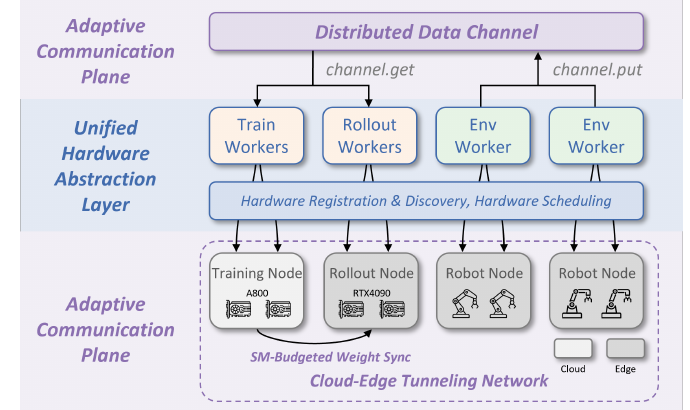
Real-world RL treated as a scheduling problem
The paper’s framing is that real-world online learning is mostly a systems problem. The real constraints are physical:
- The robot is the bottleneck, so it should never sit idle waiting for the learner.
- Hardware is heterogeneous: different arms, cameras, and edge versus cloud GPUs.
- Networks cross administrative domains: NATs, campus networks, factory VLANs.
- Experiments run for days, so they get interrupted.
Earlier systems such as SERL and QT-Opt handle one robot (or a few identical ones) with a synchronous or hand-wired pipeline. USER’s answer is to borrow the large-scale RL framework machinery that already exists for GPUs, and to extend its resource model so that robots fit in it too.
A robot is just another rank
This is the “Unified Hardware Abstraction Layer.” Strip the name and it’s a Kubernetes device plugin / Ray custom resource for robots:
- Hardware unit. The scheduler’s atomic allocatable thing: one GPU, or one robot bundled with its cameras and spacemouse. Each unit gets a typed descriptor plus config (IP, camera serials).
- Node group. A set of nodes with homogeneous units, such as
4090orfranka. - Rank. Just the global index of a unit within its group. Two Frankas on nodes 1–2 are
frankaranks 0 and 1. - Placement. Maps process ranks onto unit ranks. Read as
units : processes,rollout: "0:0-1"means GPU rank 0 hosts rollout processes 0 and 1.env: 0-1binds env i to Franka i.
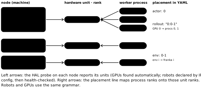
The robots get no new scheduling semantics. They just speak the same placement grammar as GPUs. The one robot-specific piece is discovery. Each hardware type supplies a HAL checker, and a probe on each node runs the checkers to build the cluster inventory. GPUs and USB cameras are found automatically. IP-bound robots are declared in config and then health-checked (is the IP reachable, are the cameras present) before they enter the schedulable pool.
Why bother: the best placement depends on the network. One rollout worker serving two envs means fewer weight-sync targets. One rollout per env cuts env↔rollout traffic. With a uniform grammar, choosing between those is a config change, not a code change.
Everything else is RLinf
Workers, channels, the placement syntax and the Ray control plane all come from RLinf (arXiv 2509.15965, same group), which was built for large-scale GPU RL. To understand how channels or placement really work, read RLinf or its repo; this paper doesn’t go into the implementation. The rest of the lineage:
- Async actor-learner. Ape-X / IMPALA / Acme-style decoupling of acting and learning.
- Buffer. Positioned against Reverb and Flashbax, which are in-memory replay services.
- Robot side. SERL’s impedance controller, task style and RLPD recipe.
- Networking. An EasyTier UDP tunnel that flattens cross-domain machines onto one TCP/IP substrate.
The network fix is channel placement, not bandwidth
The natural objection: rollout on a real robot is slow, so why optimize the network? The answer is that the cost here is latency inside the control loop, not throughput. Every step is obs → rollout → action → robot.
The cross-domain experiment puts the master and training in City A, and the rollout GPU and robot together on a LAN in City B. Inference is not in the cloud. In the baseline, though, the channel, the FIFO queue that obs and actions pass through, is hosted on the master. Every observation therefore hairpins from B to A and back to B, just to reach a GPU in the same building.
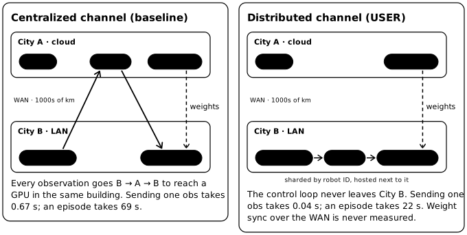
The distributed channel fix shards the queue by key (robot ID), so each shard lives next to its producer and consumer. That alone gives the ~3× shorter episode generation time (69 s → 22 s). In other words, RLinf’s default channel placement assumed one datacenter, and USER fixes that assumption.
What the network section doesn't cover
- Weight sync over the WAN. This is the traffic that actually has to cross cities, and where bandwidth matters (π0 is ~3B params). It is never measured cross-domain.
- “Consistently reduces overhead.” In the same-domain rows, send-action is slightly worse with distributed channels (0.028 vs 0.021 s).
SM-budgeted weight sync
This is the most technical-sounding knob, and it turns out to be small. NCCL collectives run as CUDA kernels, and each launches some number of CTAs (thread blocks), each occupying an SM. When new weights are broadcast to a GPU that is also running policy inference (in the example config, a single 4090 hosts both actor and rollout), the broadcast kernels take SMs away from inference, and the latency spikes land in the control loop. USER caps NCCL’s CTAs (maxCTAs in ncclConfig_t / NCCL_MAX_CTAS). The transfer gets slower, but compute stays free for rollout. It’s the same instinct as CUDA stream priorities. On a 4090 the transfer is PCIe-bound anyway, so the cap probably costs little. The paper has no ablation of it.
Full async works because every algorithm is off-policy
The pipeline lets generation, data transfer, training and weight sync overlap instead of taking turns:
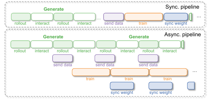
This only works cleanly because every algorithm they run tolerates stale data by construction:
- SAC, RLPD (SAC + 50% demo sampling + a critic ensemble with LayerNorm), and SAC-Flow (SAC with a flow-matching actor) are off-policy RL.
- HG-DAgger is behavior cloning on expert intervention labels.
The paper never says it, but on-policy methods like PPO or GRPO would need off-policy corrections (V-trace, or AReaL-style decoupled clipping) to use this pipeline.
Two results are worth remembering, both on peg insertion with a CNN policy:
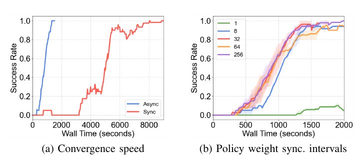
- (a) Wall-clock convergence drops from 8000+ s to ~1500 s. This is the real result. The headline “5.7× / 4.6× training throughput” (Table V) mostly means the learner no longer waits for episodes, so it takes more gradient steps on the same data, which raises the update-to-data ratio. Episode generation only speeds up 1.2× (π0) and 1.55× (CNN).
- (b) The staleness worry runs backwards. Syncing weights every update makes training diverge. Intervals of 32–256 are all fine, and the default config uses ~30. With action chunks, a policy that changes mid-episode hurts more than a policy that lags. The interval appears to be counted in learner updates, so its wall-clock meaning depends on update cost. π0 HG-DAgger uses interval 1, but a π0 update takes ~6 s.
The buffer is tiered storage
It works as follows:
- An in-memory index of every sample, with metadata (policy version, timestamp, episode ID).
- Async writes of trajectories to disk.
- A bounded FIFO cache of recent samples in RAM.
- Transparent reloads from disk on a cache miss.
Sampling throughput scales with the cache ratio r = cache / buffer size. A pure in-memory buffer is fastest, a pure on-disk buffer gets less than half of that, and USER sits in between with unbounded capacity.
The motivation is long-horizon, multi-session training. Their demo is a two-day π0 DAgger run: day 1 trains on a red duck, and day 2 adds three new objects. With the persistent buffer, the red duck stays at 10/10. With a small non-persistent buffer that evicted day-1 data, it drops to 6/10.
What the buffer section leaves open
- Capacity vs persistence. The forgetting experiment compares against a small buffer, so a large in-memory buffer would likely give the same result. It shows that replay prevents forgetting, not that persistence specifically does. It’s also 10 trials per object.
- Sampling distribution. If sampling is uniform over all indices, the cache hit rate is ≈ r. That’s all Fig. 14a shows.
- Policy-aware sampling and crash recovery are described but never exercised.
What it leaves out: the actual rollout bottleneck
In practice, the slow parts of a real-robot RL loop are weight sync and fast inference. A fast rollout usually means TensorRT, and engine conversion is slow. USER never touches the inference-optimization side. Its rollout is plain PyTorch, at 0.21 s per π0 chunk, which is slow for a 10 Hz loop. So the conversion problem never comes up in the paper. The options, from least to most work:
- Sync less often. The paper’s own Fig. 16b says larger intervals are more stable for off-policy setups. Conversion then becomes one more async stage: build the new engine in the background and swap it in at an episode boundary.
- TensorRT refit. Build the engine once as refittable, then push new weights through the refitter (seconds, not minutes). The cost is that refittable engines block some optimizations that fold weights into constants. INT8/FP8 adds a separate problem: refitting doesn’t redo calibration, so scales drift unless they are recomputed.
- CUDA graphs with in-place weight copy. Capture once with static parameter buffers, then
copy_()new weights into the same memory, and the graph stays valid. There is no conversion step at all, at the cost of TRT’s fusion. This fits flow-matching policies well, since a fixed number of denoising steps captures cleanly as a graph.
Results and fine print
Setup and headline numbers
- Tasks. Five Franka tasks: peg insertion, charger plugging, cap tightening, pick-and-place, and table clean-up.
- Hardware. Small policies (ResNet CNN, flow) train on one RTX 4090. π0 gets full-parameter training on 4×A100.
- RL results. SAC, RLPD and SAC-Flow reach near-100% on peg and charger in ~2000 s. Training speed is comparable to or faster than SERL on the same tasks.
- π0 with HG-DAgger. Pick-and-place goes from 39/60 to 58/60, and table clean-up from 9/20 to 16/20.
- Multi-robot. Four Frankas at two sites 3 km apart all converge in ~2600 s. A Franka and a 6-DoF ARX train one shared CNN policy, after the observation and action spaces are unified into the end-effector frame.
- Rewards. Rewards can be rule-based (pose distance), binary labels from a human foot pedal, or a ResNet18 success classifier. The classifier matches human labels on peg insertion.
Rough edges
- The abstract claims simulation experiments, but the body reports only real-robot ones.
- Table V has visible slips: π0 async send-data reads “7.903(±)”, identical to its training period, and the CNN+SAC sync training-period std is larger than its mean.
- The evaluations are small (10–60 trials).