Written by Claude Opus 5.5 (
claude-opus-5-5) from a discussion of the paper.
SERL is an open-source, full-stack kit for running RL directly on a real robot arm from camera images. Its central bet is that real-world robot RL is held back by implementation, not algorithms, and the paper says so outright: the goal is “not to propose novel algorithms or tools.” Almost every learning component is borrowed, much of it from the same Berkeley lab. What the paper adds is careful assembly, one genuinely useful controller trick, and an empirical claim: put together carefully, the stack learns a sub-millimeter PCB connector insertion from wrist-camera images, reaching 100/100 success in about 20 minutes of real-world training.
The method, end to end:
- Inputs: 20 teleoperated demos (SpaceMouse), plus a reward. The reward is either hand-coded from the end-effector pose or a binary success classifier on images. Hardware is a Franka arm with two wrist cameras.
- What’s trained: an RLPD agent (a soft actor-critic variant) with an ImageNet-pretrained ResNet-10 encoder and a 2-layer MLP. Training is online. Demos sit in their own buffer, and each batch is half demos, half online data. Acting and learning run as separate processes.
- At run time: at 10 Hz, the policy outputs a 6D delta pose, a twist in the current gripper frame. A 1 kHz impedance controller tracks it.
- The one non-standard operation: inside that 1 kHz loop, the controller’s target is clamped to within Δ of the arm’s measured position. That caps contact force without any force sensor, so random exploration can’t crush the PCB.
The controller’s error is the force
An impedance controller is a virtual spring-damper:
It does not measure force. It generates force from the gap between where the arm is (p) and where it’s been told to be (p_ref). The target p_ref comes from the policy. Every 100 ms the policy says something like “move 2 cm down,” p_ref is set to the current pose plus that move, and the result is interpolated up to 1 kHz.
That’s a problem specifically for RL. Say the arm is at z = 5 cm, the table surface is at 3 cm, and the policy says “down 4 cm,” so p_ref = 1 cm. The arm hits the table at 3 cm and stops, leaving e = 2 cm, so the spring presses into the table with k_p × 2 cm. An exploring policy keeps saying “down,” so p_ref keeps sinking, e keeps growing, the push keeps growing, and the pins bend.
The fix is to clamp the target every 1 ms tick, so p_ref is never more than Δ from the measured p. Then the spring force can never exceed about k_p·Δ, whatever the policy asks for. For example, k_p = 2000 N/m and Δ = 1 cm gives about 20 N.
"I should have reached x, but only reached y"
That reading of e is right in steady contact: when the arm is stopped and pressing, the surface pushes back with exactly k_p·e. But the controller isn’t using e to detect anything. It produces force from e, so keeping e small keeps the force small. The force is bounded by construction, not measured and then reacted to.
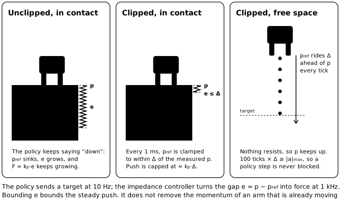
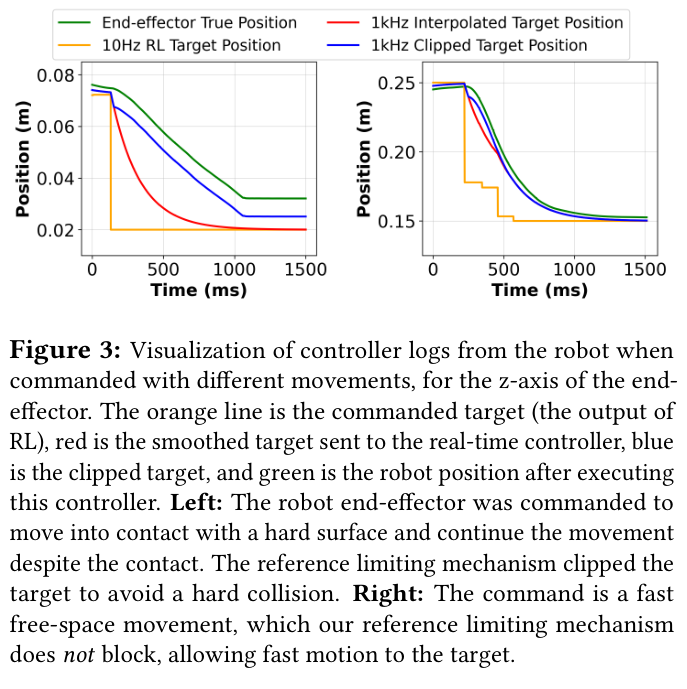
The paper’s controller logs show both cases on real hardware. In contact (left), the clipped target (blue) hugs the stalled arm, even though the policy’s target (orange) is far below. In free space (right), the clipped target never gets in the way of fast motion.
\begin{algorithm}
\begin{algorithmic}
\FOR{each policy step (10 Hz)}
    \STATE $a \gets \pi(\text{wrist images}, \text{proprio in } b_0 \text{ frame})$ \COMMENT{6D twist, gripper frame}
    \STATE $p_{goal} \gets p + a$
    \FOR{$M = 100$ ticks (1 kHz)}
        \STATE $p_{ref} \gets$ interpolate toward $p_{goal}$
        \STATE $p_{ref} \gets p + \mathrm{clip}(p_{ref} - p, -\Delta, \Delta)$ \COMMENT{the trick: relative to measured $p$}
        \STATE apply $F = k_p (p_{ref} - p) - k_d \dot p + F_{ff} + F_{cor}$ via $J^\top$
    \ENDFOR
\ENDFOR
\end{algorithmic}
\end{algorithm}
Why clip there, and not somewhere else
- Not on the policy’s action. A PCB tolerates only a tiny force, so Δ ends up on the order of micrometers. Limiting the policy to micrometer steps would make episodes impossibly long. Clipping in the 1 kHz loop doesn’t slow free-space motion as long as M·Δ ≥ |a|ₘₐₓ, because 100 ticks of Δ cover one policy step.
- Not by lowering the gains. A softer spring caps force too, but it ruins tracking accuracy everywhere.
- Not with a wrist force/torque sensor. The paper’s stated reasons are practical: noise, calibration, and hardware cost. The more fundamental difference is that a sensor threshold is reactive (detect excess force, then respond), while clipping is preventive (the excess force is never commanded in the first place).
What the clip doesn’t do
It caps the steady push, not the impact
Clipping limits how hard the arm keeps pressing after contact. It does nothing about the momentum of an arm that’s already moving fast: impact force depends on velocity, effective mass, and the stiffness of whatever gets hit, and none of that is removed by limiting the target. The damping term is the velocity-dependent part, and its paper bound, 2k_d·Δ·f with f = 1 kHz, is very loose. So the clean guarantee really covers only the spring term.
In practice the arm is slow (small actions at 10 Hz, roughly 0.1 m/s), so this is a “don’t destroy the PCB or the robot while RL explores” mechanism, not a human-safety one. Human safety on a Franka comes from separate layers: its built-in collision reflexes and speed/force limits. Franka’s collision detection is the “expected vs. actual” idea: it compares the joint torques its dynamics model predicts against the torques it measures.
The relative frame works because every input rides with the gripper
The second design choice behind the robustness claims is to express everything relative to the gripper:
- Start pose. At the start of each episode, the end-effector pose b₀ is randomized uniformly within a box: 10×10 cm for PCB, 20×20 cm for cable routing.
- Proprioception is expressed relative to that start pose: .
- Actions are twists in the current gripper frame.
The proprioception therefore tells the policy “how far I’ve moved since the episode started,” not “where I am on the table.” The policy can’t memorize “go to (x, y, z),” so it has to find the target in the images. Randomizing the start pose is equivalent to physically moving the target every episode, without ever moving it. That’s why the trained policies keep working when the target is moved in the middle of an episode.
Only because the cameras are on the wrist
PCB insertion and cable routing use two wrist cameras and no fixed camera (Table 2). The Figure 1 photos are for the paper, not what the robot sees. Wrist images, start-relative proprioception, and gripper-frame actions all live in the same gripper-centric world: “the socket is to my left in the image” means “move left in my frame,” wherever the arm is.
A fixed head or side camera would break this. Its image encodes the arm’s absolute position, so the network could learn “go to that spot in the image” and fail when the target moves. Object relocation, the one task with a side camera, is also the one task without randomized start poses (it resets above the bin center), and the paper makes no relative-frame robustness claim for it.
Everything else is borrowed
- RL algorithm: RLPD (Ball et al., 2023). SAC with a high update-to-data ratio, 50/50 sampling between the demo buffer and the online buffer, and LayerNorm in the critic so that the high update-to-data ratio doesn’t destabilize training. Off-policy RL is what makes 20 minutes possible.
- Rewards, three options:
- Hand-specified. PCB uses the end-effector pose, valid because the connector is held rigidly in the gripper.
- Binary classifier. Trained on images, with r(s) = log p(success | s).
- VICE (Fu et al., 2018). Every state the policy visits is added to the classifier’s training set as a negative, which stops the policy from exploiting the classifier. This makes the setup GAN-like: the policy is the generator and the classifier is the discriminator.
- Reset-free training with forward/backward agents (Han et al., Gupta et al., Sharma et al.). Two independent agents, each with its own policy, Q-function, and reward. The forward agent does the task, and the backward agent undoes it, returning things to the starting state. Used for object relocation, where the strawberry has to go back into the original bin.
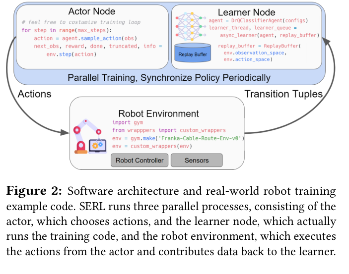
- Separate actor and learner processes. The actor keeps a fixed control rate (which matters for contact and deformables), while the learner trains at a high update-to-data ratio and syncs weights periodically.
Results
Implementation snapshot, likely to date
Task Rewards Training RL success BC success (100 demos) Cycle time RL / BC PCB insertion ground-truth pose 20 min 100/100 10/100 5.2 s / 10.1 s Cable routing classifier 31 min 100/100 19/100 4.1 s / 13.6 s Object relocation (fwd + bwd) classifier 105 min 100/100 58/100 7.5 s / 18.9 s RL starts from 20 demos, while BC gets 5× as many (100). Everything trained on a single RTX 4090. RL policies also beat the human teleoperators’ cycle times, by up to 3×. As a reproducibility check, a team at the University of Washington set up a peg insertion task in under 3 hours, and it converged in 19 minutes to 100/100.
So the evidence is “it works, and others can reproduce it,” which is the right evidence for a systems paper. Most robot RL results never get reproduced because nobody can rebuild the setup. SERL became the foundation for HIL-SERL, which adds human corrections during training and tackles much harder tasks on the same stack.
What the results lean on
- No ablations. The thesis is “the details matter,” but the paper never removes reference clipping, the relative frame, or the 50/50 demo sampling one at a time to show which details carry the result.
- The BC baseline is weak. It’s a ResNet-10 + MLP behavior cloner, not Diffusion Policy or ACT, both of which already existed. “10× better than BC” partly measures the baseline.
- Table 1 (comparison with prior insertion systems) isn’t apples to apples. The rows use different robots, tasks, and tolerances, and the authors acknowledge this.
- Narrow distributions. Start regions are 10–20 cm boxes, each task has one object, and evaluation uses the training distribution. “100/100” means very reliable on this setup, not general.