Variational Autoencoder

We’ll approach VAE with two prospective: one from intuition and engineering, which is based on this Blog post: all my images are from the blog. The other perspective is from Carl Doersch’s tutorial on variational autoencoders. Note how we did not approach the original paper as its framing can be hard to understand without prior knowledge.

The intuition

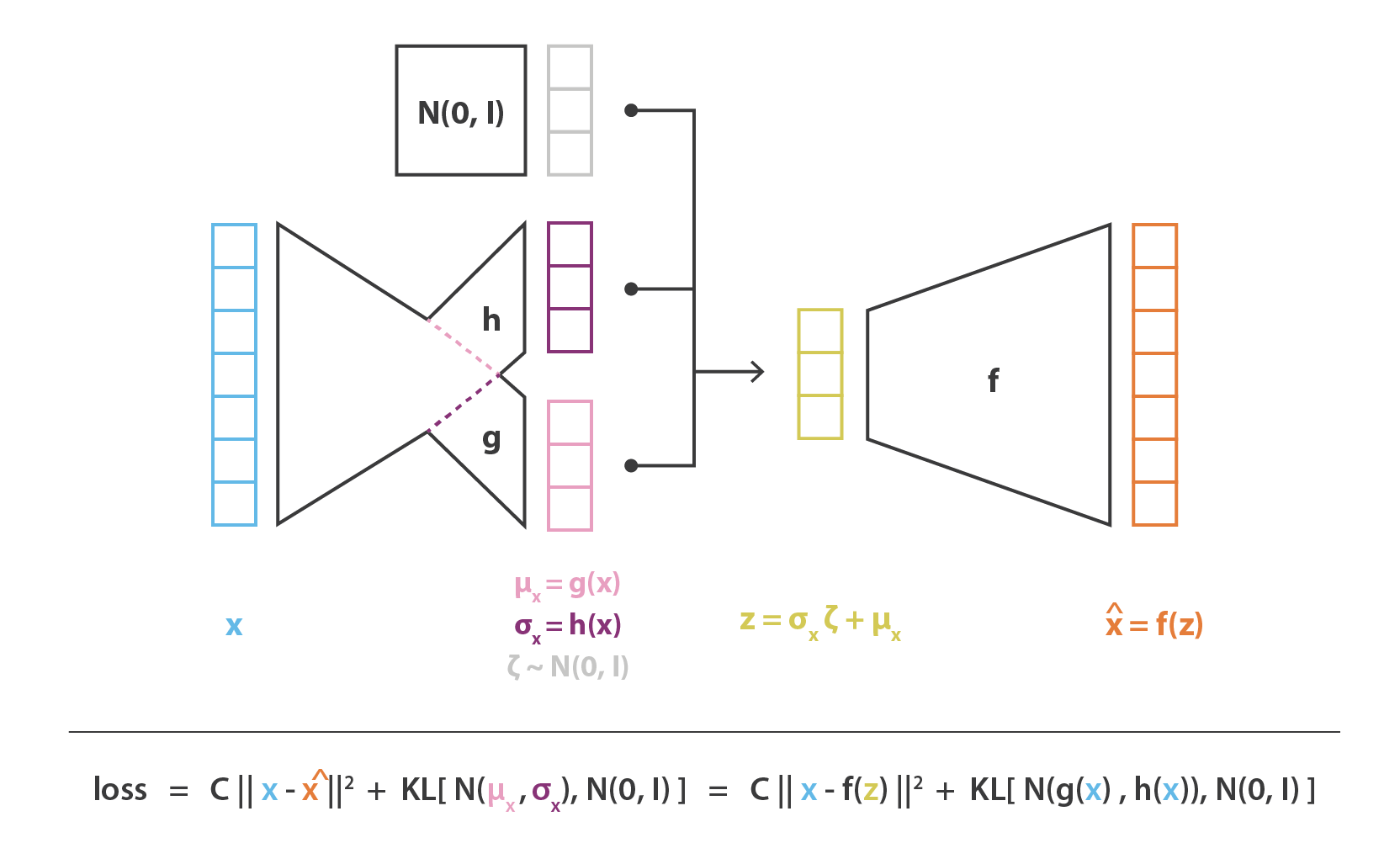
Auto encoder: easy, but may not produce what we want

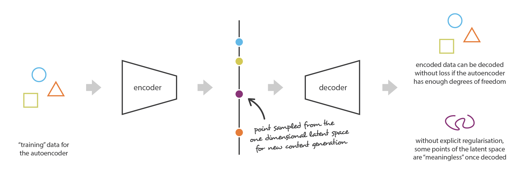
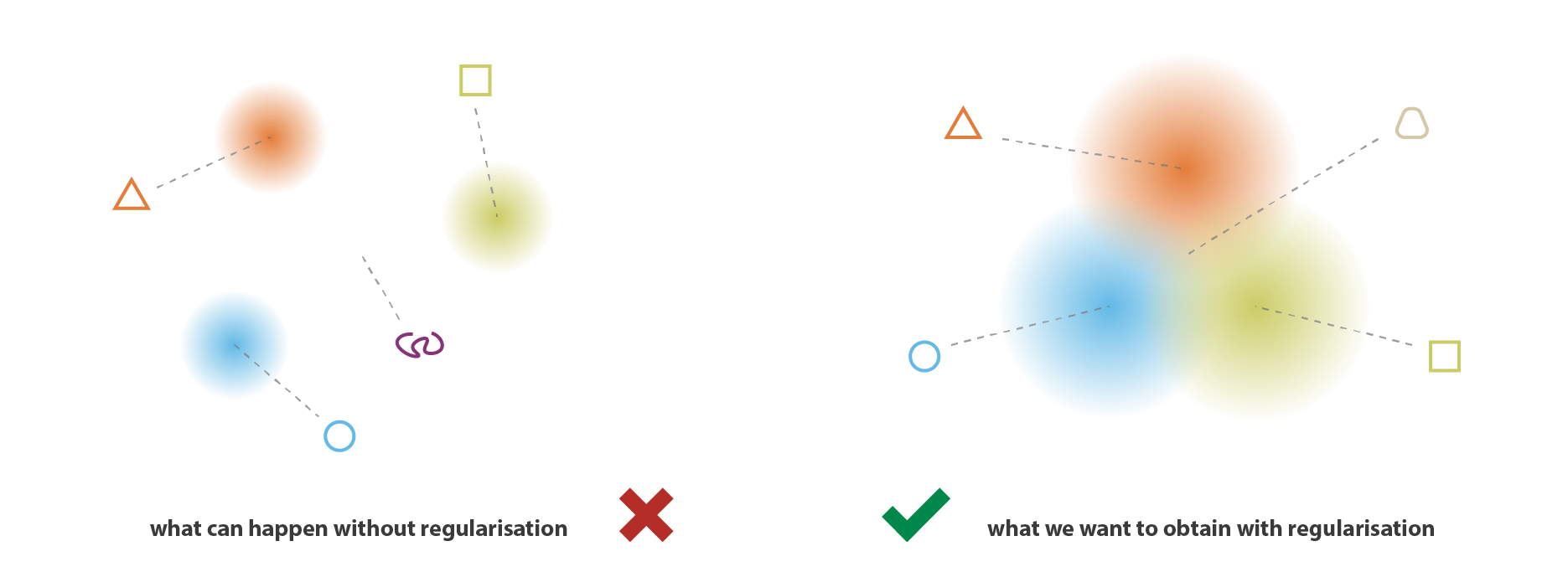
A variational autoencoder can be defined as being an autoencoder whose training is regularised to avoid overfitting and ensure that the latent space has good properties that enable generative process.

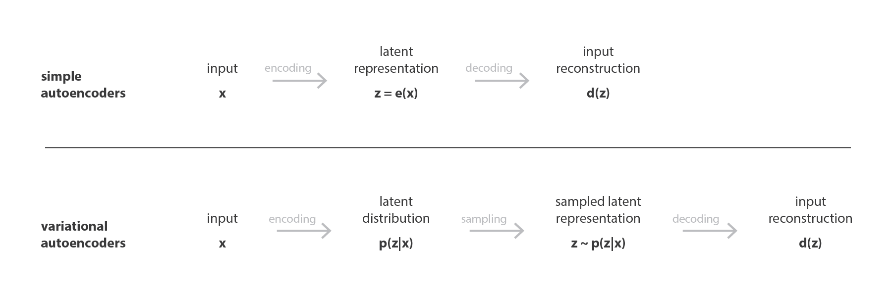
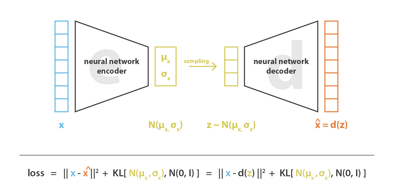
We want the distribution of encoder similar to a standard normal distribution (input → distribution → almost normal).

Note that $\mu$ and $\sigma$ are both multi-dimension embeddings.

---

The rest of the note starts from me reading the tutorial, discuss with ChatGPT 5.5 Pro, and then feeding the history to Claude Opus 4.7 with a follow up discussion.

---

Why introduce $z$ at all

The intuitive AE→VAE story leaves a gap: why have a latent variable in the first place? The generative-model framing makes this clear.

VAE doesn’t model $p(x)$ directly. It models data as the visible result of hidden causes:

$$z\sim p(z),x\sim p_{\theta }(x|z)$$

Two reasons this matters:

1. Modeling complex $p(x)$ through a simpler latent space. $p(x)=\int p_{\theta }(x|z)p(z),dz$ — instead of fitting the data distribution directly, fit a decoder conditioned on a simple prior. Standard hierarchical modeling.
2. Controlled generation. With a fixed prior $p(z)=\mathcal{N}(0,I)$, sampling new data is just: draw $z\sim \mathcal{N}(0,I)$, decode. Plain autoencoders don’t have this — their latent space is unconstrained, so a random point in latent space may decode to nonsense.

The probabilistic framing immediately forces a question: given observed $x$, what $z$ produced it? That’s $p_{\theta }(z|x)$, and it’s intractable because computing it via Bayes’ rule needs $p(x)=\int p_{\theta }(x|z)p(z),dz$ — the very integral we couldn’t do in the first place. This is the source of all the variational machinery below.

The probabilistic perspective (Doersch’s formula 5)

The central equation in Doersch’s tutorial:

$$\log p_{\theta }(x)-D_{KL}(q_{\varphi }(z|x)|p_{\theta }(z|x))={\mathbb{E}}_{q_{\varphi }(z|x)}[\log p_{\theta }(x|z)]-D_{KL}(q_{\varphi }(z|x)|p(z))$$

The right-hand side is the ELBO — the VAE training objective. Decomposed:

• ${\mathbb{E}}_{q_{\varphi }(z|x)}[\log p_{\theta }(x|z)]$ — reconstruction term. Sample $z$ from the encoder, decode, score how well it reconstructs $x$.
• $D_{KL}(q_{\varphi }(z|x)|p(z))$ — regularizer. Keep the encoder’s output distribution close to the prior. This is what forces the latent space to be organized for generation.

Translation back to the architecture:

Symbol	Meaning	Neural net role
$x$	datapoint	input
$z$	latent	bottleneck code
$p(z)$	prior	usually $\mathcal{N}(0,I)$
$p_{\theta }(x\Vert z)$	decoder likelihood	decoder network
$p_{\theta }(z\Vert x)$	true posterior	the intractable thing
$q_{\varphi }(z\Vert x)$	approximate posterior	encoder network output

The left-hand side is the thing we wish we could optimize: $\log p_{\theta }(x)$ minus the (unknown) gap between our approximation and the true posterior. The right-hand side is what we can optimize. Maximizing the right-hand side simultaneously:

• Pushes $\log p_{\theta }(x)$ up (decoder + prior fit the data better),
• Tightens the bound by pulling $q_{\varphi }$ toward $p_{\theta }(z|x)$ — without ever computing the gap.

See ELBO for the full derivation, the “gap shrinks for free” argument (gradient w.r.t. encoder params is exactly minus the gradient of the gap), and why the KL is in the direction $q|p$ rather than $p|q$. See Amortized variational inference for why one network $\varphi$ handles all datapoints, and the cost — the amortization gap, which connects to posterior collapse.

Training: the Reparameterization trick

The encoder outputs ${\mu }_{\varphi }(x)$ and $\log {\sigma }_{\varphi }^2(x)$. To sample $z\sim q_{\varphi }(z|x)$ while keeping the operation differentiable:

$$z={\mu }_{\varphi }(x)+{\sigma }_{\varphi }(x)\odot ϵ,ϵ\sim \mathcal{N}(0,I)$$

Gradients flow through $\mu$ and $\sigma$ into the encoder. Without this, you can’t backprop through the sampling step — see Reparameterization trick for why and what to do when $z$ is discrete (the case motivating VQ-VAE’s straight-through codebook lookup).

For diagonal Gaussian $q_{\varphi }$ against an $\mathcal{N}(0,I)$ prior, the KL has a closed form:

$$D_{KL}(\mathcal{N}(\mu ,\mathrm{diag}({\sigma }^2))|\mathcal{N}(0,I))=\frac{1}{2}\sum _i\left({\mu }_i^2+{\sigma }_i^2-\log {\sigma }_i^2-1\right)$$

so the training loss is a sum of reconstruction (typically MSE or BCE depending on the likelihood model) and this closed-form KL. No Monte Carlo estimate needed for the KL — only for the reconstruction term, which uses a single $ϵ$ sample per datapoint in practice.

Positioning: VAE vs GAN vs Flow Matching

Three ways to set up a generative model. The clarifying axis: does the model need to invert $x\mapsto z$?

Model	Latent randomness	Encoder / amortized posterior	Training objective
VAE	Yes, sampled at training and inference	Yes — $q_{\varphi }(z\Vert x)$	ELBO (lower bound on $\log p(x)$)
GAN	Yes, initial noise only	No	Adversarial: ${\min }_G{\max }_{D}V(G,D)$
Flow Matching	Yes, initial noise only	No	Regression on velocity field

VAE is alone in needing an encoder. The other two only map noise → data; they don’t ask “for this observed $x$, what $z$ caused it?”

• GAN has a generator $G(z)$ with no inverse. Training matches the distribution of generated samples to the data distribution via a discriminator. Avoids the ELBO entirely, but introduces adversarial-game instabilities and mode collapse — the GAN can produce sharp samples while ignoring chunks of the data distribution.
• Flow Matching reframes generation as an ODE: $d{x}_t/dt=v_{\theta }(x_t,t)$ transports noise to data. Training regresses the velocity field against conditional target velocities. The marginal/conditional flow matching equivalence is what makes this tractable — see Flow Matching. No posterior, no encoder.

VAE’s tradeoff: you pay for the encoder with an amortization gap and a lower-bound gap, but you get something the others don’t — an inference network $q_{\varphi }(z|x)$ that maps observed data to latent codes. If you want representations directly, VAE-family models give them; GAN and flow matching require post-hoc inversion procedures (GAN inversion, flow inversion via solving the reverse ODE).

For positioning against diffusion specifically: DDPM’s training objective is itself a (reweighted) ELBO on a $T$-step latent variable model with frozen forward $q$ and learned reverse $p_{\theta }$. Structurally diffusion is closer to VAE than to flow matching — hierarchical latent variable model + variational inference. See Score matching for the equivalent score-regression view of the same training loss.

Next: VQ-VAE

VAE assumes continuous latents — sampling requires reparameterization, which assumes differentiability through the sampling step. For discrete latents (token-like codes), the reparameterization trick breaks. VQ-VAE replaces the Gaussian sampler with a nearest-neighbor lookup into a learned codebook + a straight-through gradient estimator for the non-differentiable step. The discrete codes also sidestep posterior collapse (the decoder can’t easily ignore a hard categorical input) and produce token sequences that downstream autoregressive or masked models can predict directly — the foundational pattern behind a lot of modern multimodal generation.