Scaling Law

Referenced material:

• chinchilla.pdf
• hitchhikers_guide_scaling_law.pdf
• cs336_lecture_9.pdf
• cs336_lecture_11.pdf

---

Scaling law basically try to answer “How do the performance changes as we vary one or more inputs”?

Data scaling laws

The Kaplan one. Loss and dataset size is linear on a log-log plot. This can be understood as say, given a bunch of data, estimate the mean. The error

$$E[(\hat{\mu }-\mu {)}^{2]}=\frac{{\sigma }^2}{n}$$ $$\log (\text{Error})=-\log n+2\log \sigma$$

Chinchilla Scaling Laws

Based on my conversations with Claude Sonnet 4.6, summarized by Claude Opus 4.6.

The Chinchilla paper (Hoffmann et al., 2022) uses three independent approaches to estimate compute-optimal training configurations. All three converge on the same result:

$$N_{\text{opt}}\propto C^{0.5},D_{\text{opt}}\propto C^{0.5}$$

meaning compute should scale model size and data roughly equally

Approach 1: Envelope Method

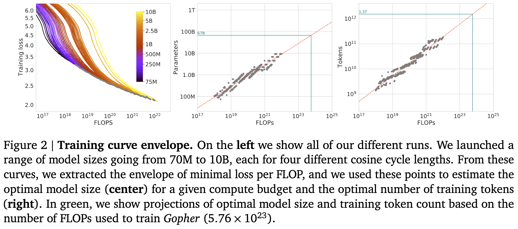
Fix a set of model sizes (70M to 10B) and for each model size, train with multiple LR decay horizons (4 per model size, spanning a 16× range). The decay horizon controls total training tokens — longer horizon means more tokens. This gives roughly ~9 model sizes × 4 horizons ≈ 36 runs.

Procedure:

1. For each run, smooth the training loss curve (Gaussian smoothing, 10-step window) and interpolate to get a continuous loss-vs-FLOPs mapping.
2. At each of 1500 log-spaced FLOP values, find which run (model size + token count combo) achieves the lowest smoothed loss — this traces the lower envelope.
3. Each envelope point gives a triplet $(C,N_{\text{opt}},D_{\text{opt}})$.
4. Plot $C$ vs $N_{\text{opt}}$ and $C$ vs $D_{\text{opt}}$, then fit power laws.

Why smooth?

Training loss is noisy step-to-step due to mini-batch variance. Without smoothing, the envelope would cherry-pick noise troughs rather than reflect the true underlying loss. The 10-step Gaussian window is narrow enough to denoise without distorting the trend.

Key trick

A single training run traces a trajectory through FLOP space. A 1B model trained for 100B tokens passes through $C=6\times 10^{18}$ on its way to $C=6\times 10^{20}$. Method 1 reuses these intermediate checkpoints as data points at multiple FLOP budgets. The complication is that a model “passing through” a FLOP budget mid-training has an LR schedule tuned for a different endpoint — hence the 4 different decay schedules per model size to partially address this.

Approach 2: IsoFLOP Profiles

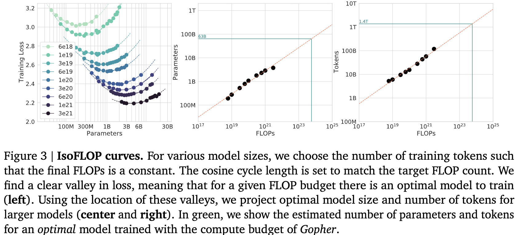
Fix a compute budget $C$, then sweep across model sizes. Since $C\approx 6ND$, each choice of $N$ determines $D=C/6N$. Train models at several $(N,D)$ points along this tradeoff and record the final loss.

Plotting loss vs $N$ at fixed $C$ gives a U-shaped curve (concave in log-log space): too-small models waste compute on excess data, too-large models starve on too little data. The minimum gives $N_{\text{opt}}(C)$.

Repeat for several FLOP budgets to get a family of IsoFLOP profiles. Read off the optimal $N$ from each, then fit $N_{\text{opt}}\propto C^a$.

Approach 1 vs Approach 2

These are nearly identical — both empirical, both find optimal $N$ for a given $C$ from the same $(N,D,L)$ data. The difference is the slice: Approach 1 takes the lower envelope across runs (IsoFLOP slices are implicit), Approach 2 explicitly groups runs by FLOP budget and finds the minimum of each U-shaped profile.

The only practical distinction is that Approach 1 reuses intermediate checkpoints across FLOP budgets via interpolation, while Approach 2 treats each run as one point — though nothing prevents doing checkpoint interpolation in Approach 2 as well.

Both assume very little (power law fit only at the end), unlike Approach 3 which posits a global parametric form $L(N,D)=A/N^{\alpha }+B/D^{\beta }+L_{\infty }$. The convergence of all three on $a\approx b\approx 0.5$ is what gives the result its credibility.

Approach 3: Just fit it

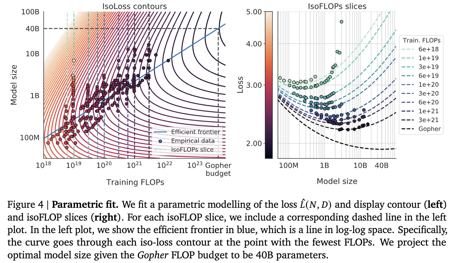
Just fit this: $\hat{L}(N,D)\triangleq E+\frac{A}{N^{\alpha }}+\frac{B}{D^{\beta }}.$ They use Huber loss + L-BFGS. According to hitchhiker guide these does not matter. It’s just fitting anyway.

Now if we say we want to find the most compute efficient model, then we’re basically fixing $\text{FLOPs}(N,D)\approx 6ND$.

WSD Schedules and Scaling Law Experiments

A major limitation of Approach 1 with cosine schedules: the LR decay horizon must match the intended training length, so you need separate runs for each token budget. WSD (Warmup-Stable-Decay) schedules fix this.

With WSD, you train one long run in the stable phase and branch short cooldowns from intermediate checkpoints. Each cooldown yields a properly-trained model for that FLOP budget. This makes Approach 1 much cleaner and more compute-efficient — the LR schedule mismatch problem disappears.