Parallelism

Data Parallel

Same model on each device, split the data.

# Sync gradients across workers (only difference between standard training and DDP)
for param in params:
	dist.all_reduce(tensor=param.grad, op=dist.ReduceOp.AVG, async_op=False)

Memory analysis

We store 5 copies of weights and 16 bytes per param.

• 2 bytes for FP/BF 16 model parameters
• 2 bytes for FP/BF 16 gradients
• 4 bytes for FP32 master weights (the thing you accumulate into in SGD)
• 4 (or 2) bytes for FP32/BF16 Adam first moment estimates
• 4 (or 2) bytes for FP32/BF16 Adam second moment estimate

Surprisingly large optimizer state.

ZeRO

Now we got some ZeRO (Zero Redundancy Optimizer)stuff:

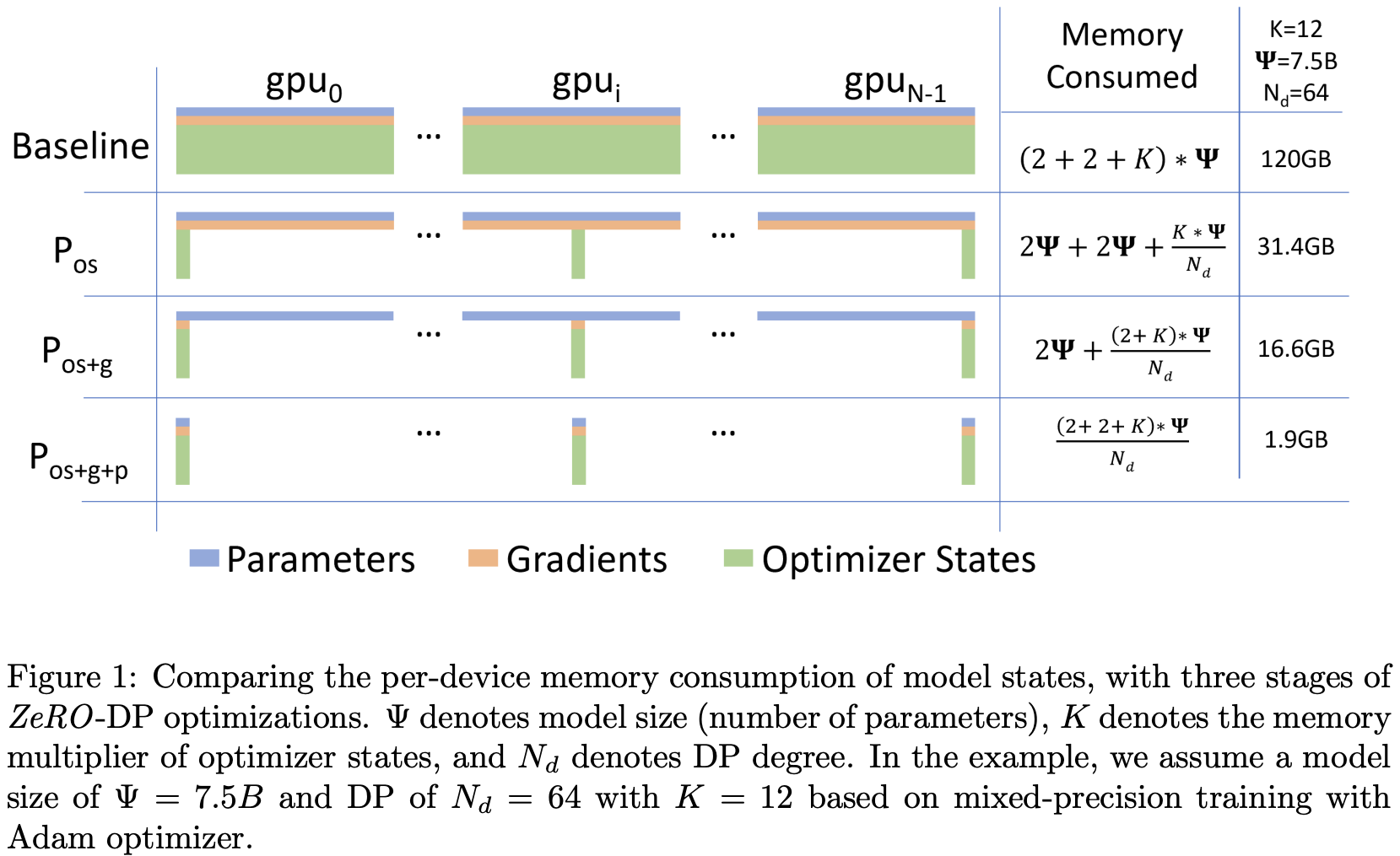
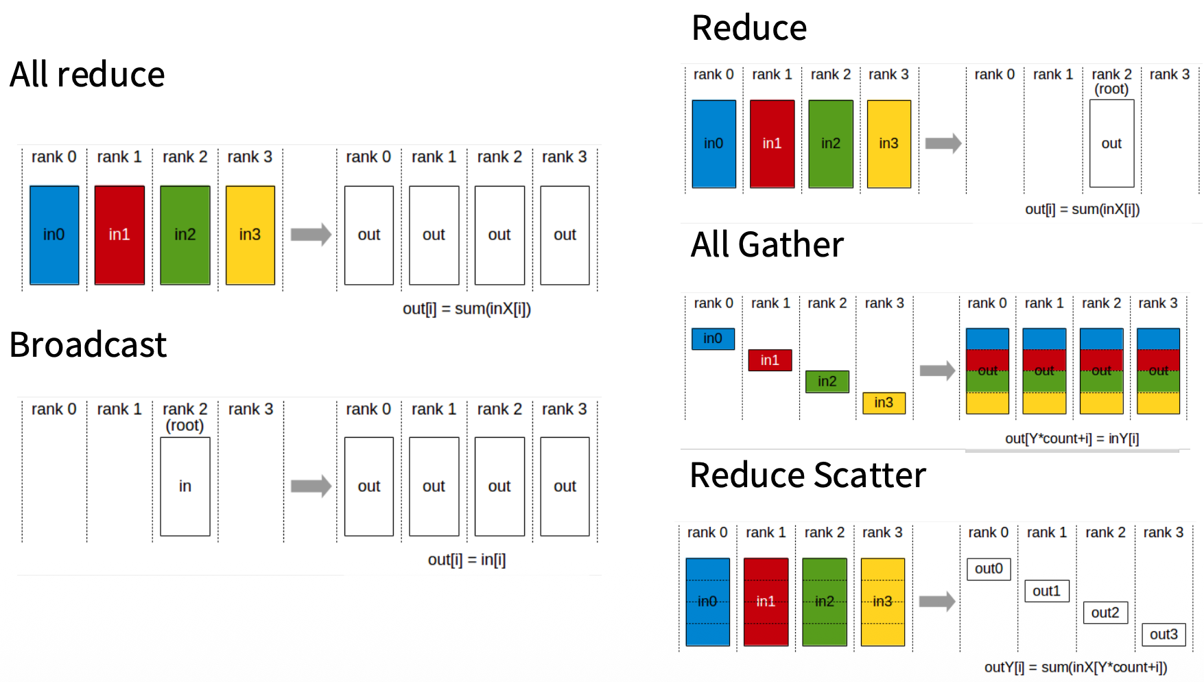
ZeRO stage 1

No need for each machine to take charge of all params. Let’s split ownership. Let’s target the optimizer state first. Each rank just take charge of the gradient of $1/N$ params (in addition to look at $1/N$ data).

• Everyone compute full gradient on their subset of the batch
• ReduceScatter the gradients. Now device $i$ has full gradient from full batch, just for the $i$ slice of params.
• Update params!
• All Gather the params so now all the devices are in sync

Same bandwidth as naive DDP

ZeRO stage 2

Shard gradient too. So replace “everyone compute full gradient” with something. We’ll need to gather the gradient from all the devices (for the whole batch), and send the params to where they belongs. So:

• Everyone incrementally goes backwards on the computation graph
  • After computing a layer’s gradients, immediately reduce to send this to the right worker (This is from slide but I thought it should be reduce scatter)
  • Once gradients are not needed in the backward graph, immediately free it
• Everyone got their slice of gathered gradient, update params!
• All Gather the params.

Still same bandwidth, (almost) free (ignoring overhead)

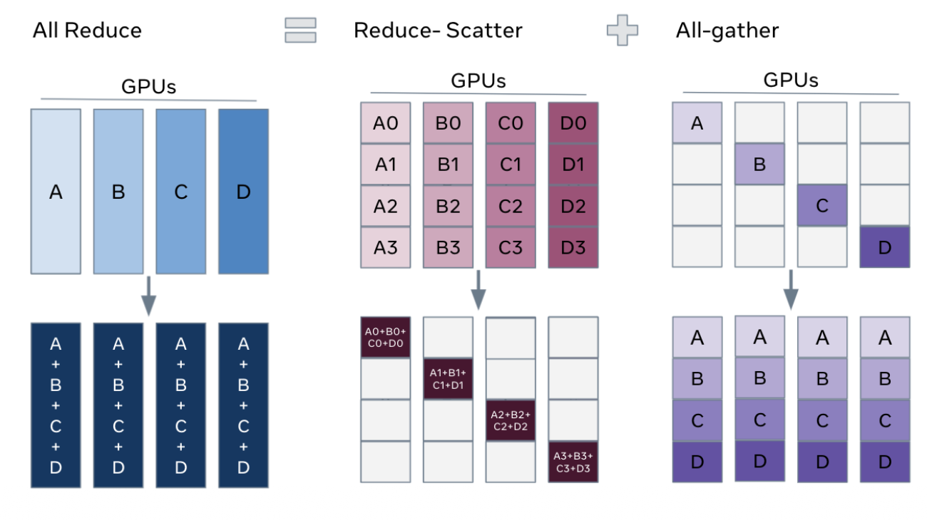
ZeRO stage 3 or FSDP

Now if we shard the param, we gonna do the forward pass somehow, or how are we going to get the “gradient for partial data”?

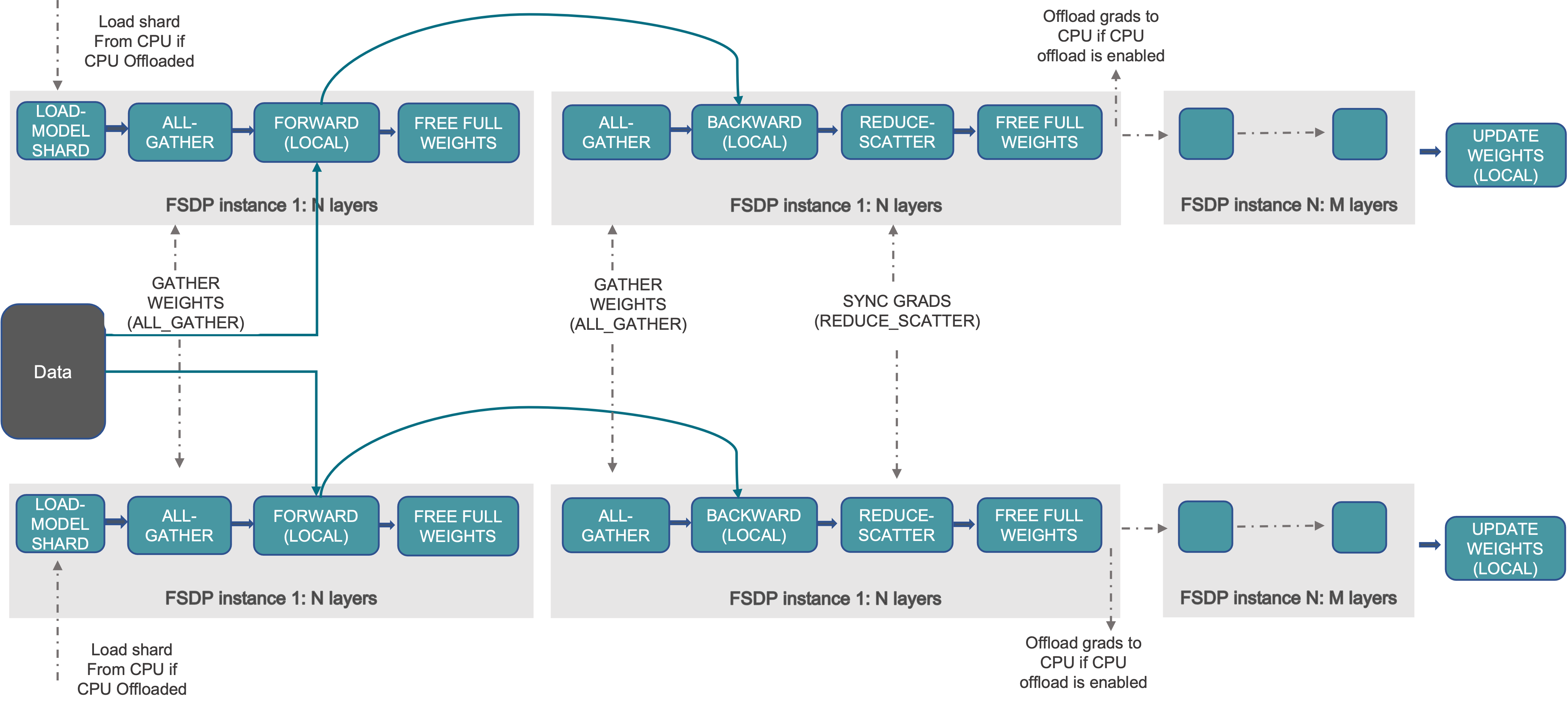
• So we go layer by layer all gather and throw the used param away (similar as stage 2 but kinda extreme) so we can still do forward / backward
• Inside backward the gradients are reduce-scattered into sharded gradients, same as stage 2.
• We can mask the communication cost by overlapping with computation.

1.5x comm cost.

Model parallelism

• Splits up the parameters across GPUs (like FSDP)
• Communicate activations (not params)

Pipeline Parallel

Layer-wise parallel cuts up layers, assigns some subset to GPUS. Activations and partial gradients are passed back and forth.

To make it faster we do CPU-like pipeline, cutting batches into smaller batches for each worker.

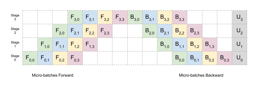
Note the “bubble” there. However, it only communicate activations and is point to point.

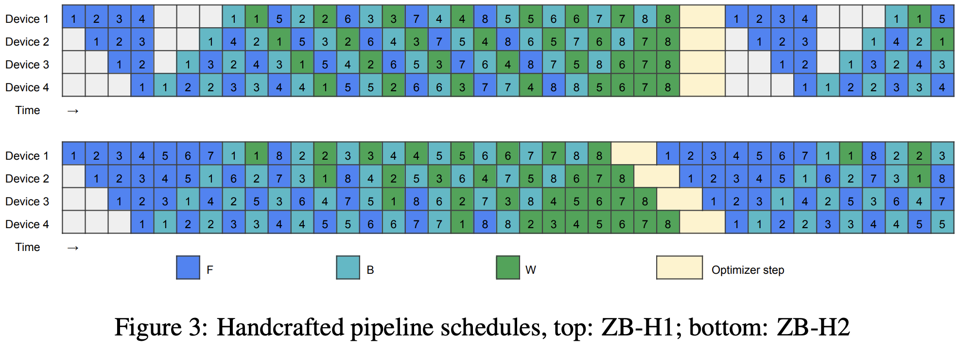
We can do better things, like using “Zero bubble” pipelining, from a 2024 ICLR paper, using the fact that the backward gradient calculation of loss w.r.t. to weight does not have dependencies and can be done whenever. So we can first compute gradient for $X$ first, then $W$.

# Split up layers
 
local_num_layers = int_divide(num_layers, world_size)
 
# Each rank gets a subset of layers
local_params = [get_init_params(num_dim, num_dim, rank) for i in range(local_num_layers)]
 
# Forward pass
 
# Break up into micro batches to minimize the bubble
micro_batch_size = int_divide(batch_size, num_micro_batches)
if rank == 0:
	# The data
	micro_batches = data.chunk(chunks=num_micro_batches, dim=0)
else:
	# Allocate memory for activations
	micro_batches = [torch.empty(micro_batch_size, num_dim, device=get_device(rank)) for _ in range(num_micro_batches)]
 
for x in micro_batches:
	# Get activations from previous rank
	if rank - 1 >= 0:
		dist.recv(tensor=x, src=rank - 1)
		
	# Compute layers assigned to this rank
	for param in local_params:
		x = x @ param
		x = F.gelu(x)
 
	# Send to the next rank
	if rank + 1 < world_size:
		print(f"[pipeline_parallelism] Rank {rank}: sending {summarize_tensor(x)} to rank {rank + 1}", flush=True)
		dist.send(tensor=x, dst=rank + 1)

Tensor Parallel

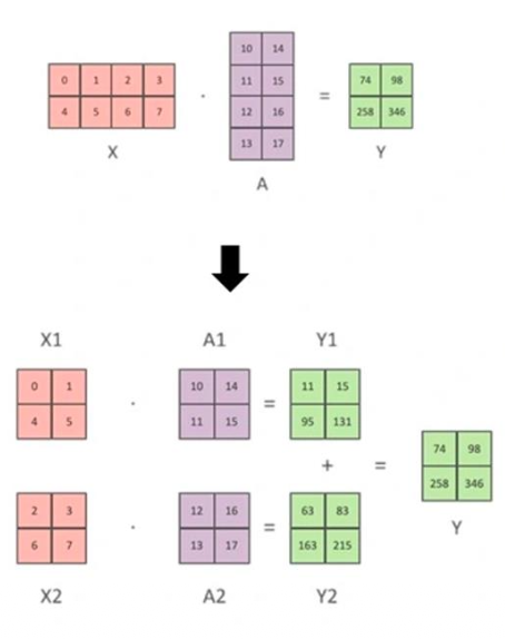
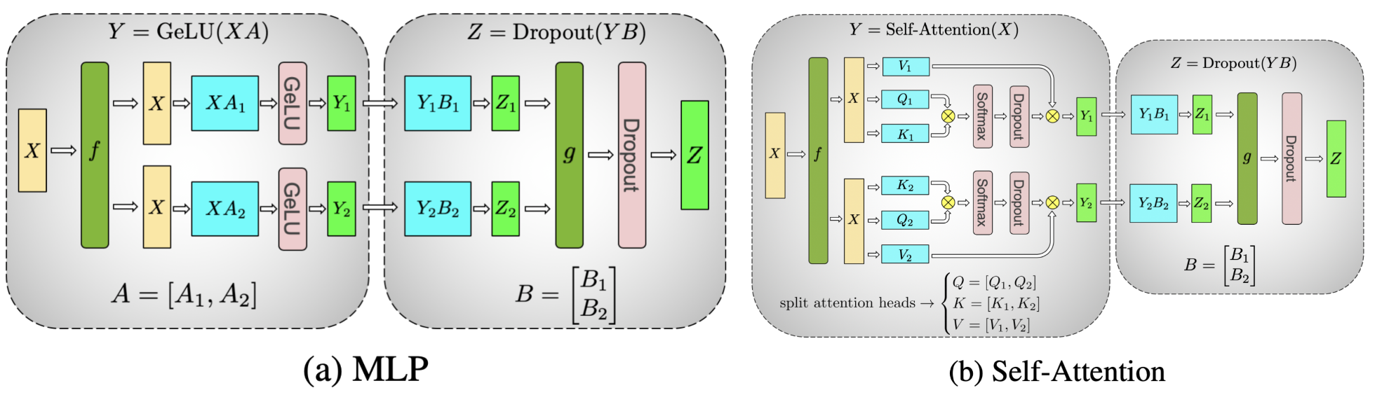
Assign columns (A1, A2) and rows (B1, B2) to separate GPUs.

• In the forward pass, f is the identity, and g is an all-reduce.
• In the backward pass, f is an all-reduce, g is the identity.

So we have no bubble and low complexity. However we need much larger communication (as this happens for all the multiplication)

local_num_dim = int_divide(num_dim, world_size) # Shard `num_dim`
# Create model (each rank gets 1/world_size of the parameters)
params = [get_init_params(num_dim, local_num_dim, rank) for i in range(num_layers)]
 
# Forward pass
x = data
for i in range(num_layers):
	# Compute activations (batch_size x local_num_dim)
	x = x @ params[i] # Note: this is only on a slice of the parameters
	x = F.gelu(x)
	
	# Allocate memory for activations (world_size x batch_size x local_num_dim)
	activations = [torch.empty(batch_size, local_num_dim, device=get_device(rank)) for _ in range(world_size)]
	
	# Send activations via all gather
	dist.all_gather(tensor_list=activations, tensor=x, async_op=False)
	
	# Concatenate them to get batch_size x num_dim
	x = torch.cat(activations, dim=1)

Sequence Parallel

Tensor Parallel only can split activations for matrix multiplies, not point wise stuff like LayerNorm and DropOut and inputs to attention and MLP. So we gonna split these too, now along sequence dim.

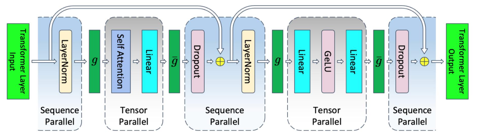
The two $g$ are either all gather or reduce-scatter.

	Sync overhead	Memory	Bandwidth	Batch size	Easy to use?
DDP/ZeRO1	Per-batch	No scaling	2 * # param	Linear	Very
FSDP (ZeRO3)	3x Per-FSDP block	Linear	3 * # param	Linear	Very
Pipeline	Per-pipeline	Linear	Activations	Linear	No
Tensor+seq	2x transformer block	Linear	8*activations per-layer all-reduce	No impact	No

3D parallelism

From DeepSpeed…

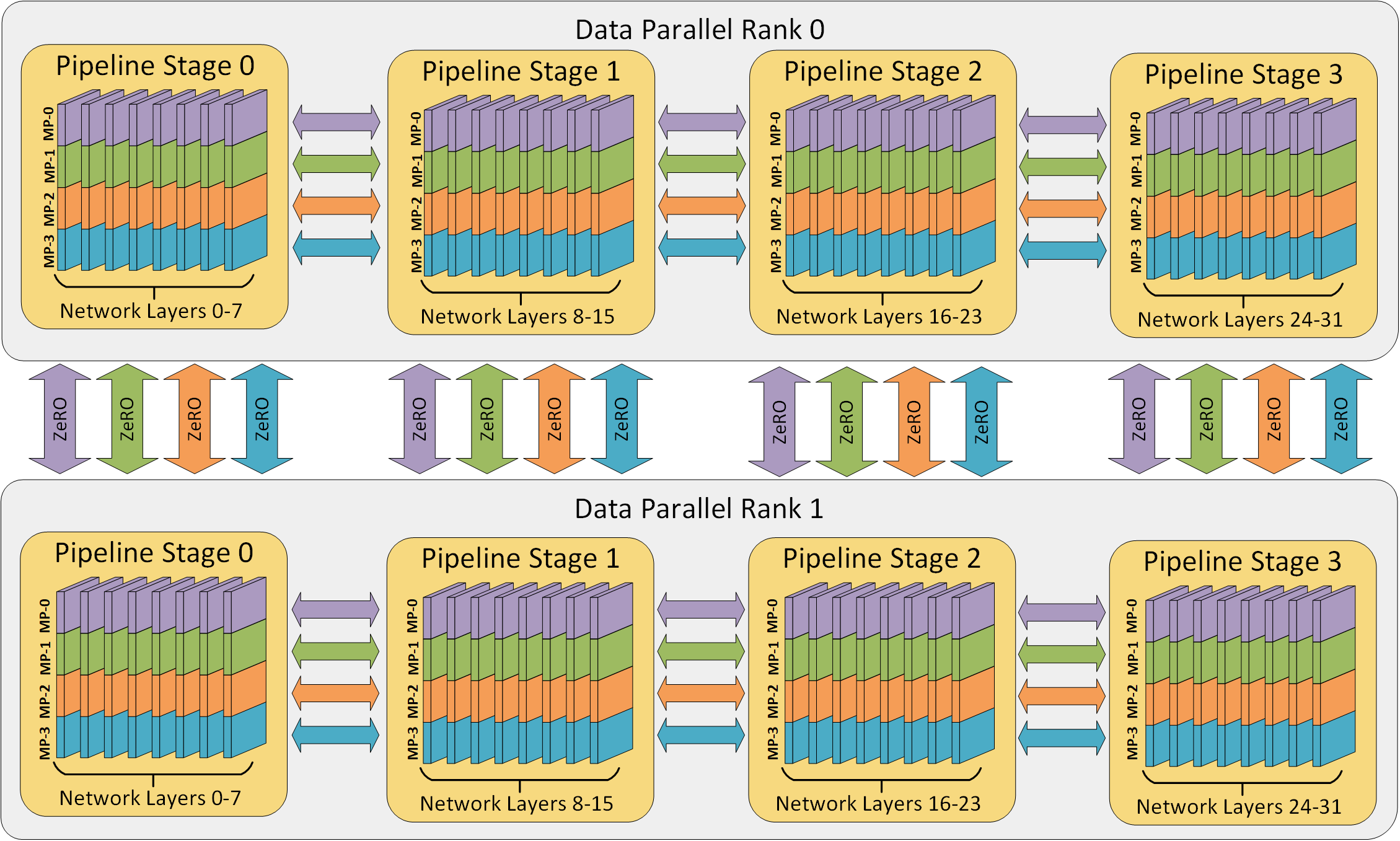
1. Until your model fits in memory..
   • Tensor parallel up to GPUs / machine
   • Pipeline parallel across machines
   • (Or use ZeRO-3, depending on BW)
2. Then until you run out of GPUs
   • Scale the rest of the way with data parallel

Strategy	What’s communicated	Frequency / blocking	Latency sensitive?	Typical placement
ZeRO (stage 3)	Params, grads, optimizer states (all-gather / reduce-scatter)	Per-layer boundary; prefetchable, not on critical path	Low–medium	Cross-node (slow links OK)
Tensor Parallel	Partial activations (all-reduce after every matmul)	Every matmul, every layer; fully blocking, cannot pipeline	Very high	Intra-node only (NVLink)
Pipeline Parallel (1F1B)	Activations between adjacent stages (point-to-point)	At micro-batch boundaries; blocking per stage, bubble overhead	Medium	Cross-node OK
DDP (baseline)	Gradients only (all-reduce once per step)	Once per step; overlapped with backward	Low	Cross-node

Bonus: Ring All-Reduce

This part is from a conversation with Claude Sonnet 4.6.

Goal

Every rank starts with a local tensor (e.g. gradients). The goal is for every rank to end up with the elementwise sum across all ranks — without any single node being a bottleneck.

Concrete Setup

4 ranks, each holding a length-4 tensor (arange(4) + rank):

Rank 0: [0, 1, 2, 3]
Rank 1: [1, 2, 3, 4]
Rank 2: [2, 3, 4, 5]
Rank 3: [3, 4, 5, 6]

Target (elementwise sum): [6, 10, 14, 18]

Each tensor is split into world_size chunks. Each rank is responsible for fully reducing one chunk.

---

Phase 1: Reduce-Scatter

Logically arranged in a ring:

Rank 0 → Rank 1 → Rank 2 → Rank 3 → (back to Rank 0)

At each step, every rank simultaneously sends one chunk to its right neighbor and receives one chunk from its left neighbor, accumulating (adding) as it goes. Notation: a/b/c/d = chunk index (0/1/2/3), subscript = source rank.

Step	R0 → R1	R1 → R2	R2 → R3	R3 → R0
1	a0	b1	c2	d3
2	d0+d3	a1+a0	b2+b1	c3+c2
3	c0+c3+c2	d1+d0+d3	a2+a1+a0	b3+b2+b1
hold	b0+b1+b2+b3 ✓	c1+c2+c3+c0 ✓	d2+d3+d0+d1 ✓	a3+a0+a1+a2 ✓

After world_size - 1 steps, each rank holds one fully-reduced chunk:

Rank 0 receives: a (chunk0) fully reduced = 0+1+2+3 = 6
Rank 1 receives: b (chunk1) fully reduced = 1+2+3+4 = 10
Rank 2 receives: c (chunk2) fully reduced = 2+3+4+5 = 14
Rank 3 receives: d (chunk3) fully reduced = 3+4+5+6 = 18

Each step moves size / world_size data. Total sent per rank:

$\text{size}\times \frac{worl{d}_{s}ize-1}{worl{d}_{s}ize}\approx \text{size}$

---

Phase 2: All-Gather

Each rank now forwards its fully-reduced chunk around the ring (no accumulation, just copy). After another world_size - 1 steps, every rank holds the complete result [6, 10, 14, 18].

Same data volume as phase 1: another ≈ size per rank.

---

Total Communication Cost

	Per-rank data sent	Total across all ranks
Naive (everyone → everyone)	O(N · size)	O(N² · size)
Ring all-reduce	≈ 2 · size	O(N · size)

The 2x comes from the two phases (reduce-scatter + all-gather). Adding more GPUs does not increase per-device communication cost — it scales linearly, not quadratically.

---

Why a Ring?

The ring topology is an implementation choice, not fundamental to reduce-scatter. The same total data is moved regardless of topology. The ring’s advantage:

• Every rank is simultaneously sending and receiving at every step — no idle ranks
• Each network link is used by exactly one sender per step — no contention
• Perfectly pipelined and load-balanced

The core idea (each rank responsible for reducing one chunk, receives that chunk from all others) works with any topology — the ring just maximizes bandwidth utilization.