A Frankenstein paper. That said, unlike the other Frankenstein paper like DINOv2, it does have stuff novel and interesting. This is a paper from Torc that targets long range scenarios. The problem here is dense BEV become too expensive. So they go sparse attention all the way. They also use self supervised learning but it doesn’t seem that important here.
Camera encoder
TL; DR: Sparse depth-enhanced multi-scale encoder.
We project each lidar point onto the camera frame for each camera. That gives sparse image . It’s then passed into Vim together with a camera embedding, derived from the intrinsic and extrinsic calibration matrix. We are then able to get a bunch of feature maps at different scales. Then these feature map (again) are fed into FPN, so now they are fused multi-scale.
Depth estimation
TL; DR: Get dense depth map from spare lidar and image.
Why we do depth estimation here? It’s used later for projecting image to 3D. What’s the author doing? First projecting lidar to image, and then the other way around. (Well, this does get richer information because the depth information is denser) But whatever. The input is the sparse lidar point cloud and the output is a dense depth image. So you can imagine this as a depth completion task. And well, as you might already know, the author just likes to put random stuff together, so they didn’t use a normal way of estimating this. Instead, they use an RNN and diffusion-like methods. I don’t think this is important. I put the detail in Appendix A The wild depth estimation method.
Lidar encoder and camera lidar fusion
TL; DR: Voxelize everything and extract features, multi scale.
Now we have dense depth, we can make pseudo-lidar. But don’t concat first, we’ll first encode lidar, and then combine them. The lidar points are voxelized first, then go through PointNet, then convolution with U-Net. Lidar is too dense, it have to be voxelized somehow. Remember the pseudo-lidar? We will just voxelize them the same way, and then concat them. If it’s empty for either of the modality, we’ll just append zero. Now we have in hand: Occupied voxels number of features, where each feature is a concatenation of the feature embedding and the XYZ coordinates.
Then we go through a new round of encoding following Sparseocc, and the result is some multi-scale features. You might ask “multiscale? Again?“. Yeah, but the previous multi-scale approach is used primarily to estimate depth size. Now it’s late encoding, incorporating both lidar and camera data, while projecting multiple times of course.
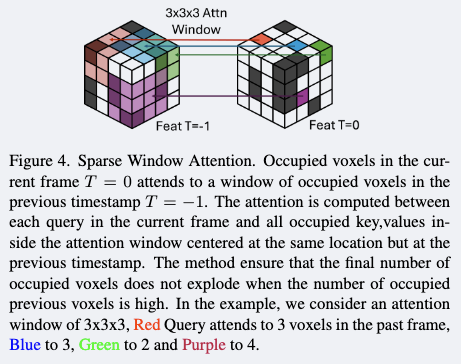
Temporal fusion
TL; DR: Current frame attend to previous frame voxels.
So far there’s Mamba, RNN and CNN. Where’s our old friend, Transformer?
We use the second smallest voxel representation and then try to align current and . First we can do a “good enough” alignment by getting from FMCW speed as well as vehicle odometry (note, extra input mentioned here).
That alignment may not be good enough. We aggregate the two frame information by sparse windowed attention.
Self supervision, the training target
TL; DR: Predict new location, get features, predict occlusion and velocity.
Self-supervision via a loss composed of a reconstruction loss for sparse occupancy and sparse velocity. They are chosen since they don’t need ground truth labels. Both take as input a four-dimensional query point , where are spatial coordinates and is time, and its outputs are both density and velocity for each queried point.
The important part is the here. We are trying to do “prediction” task. Note that our representation is heavily position based (you can’t just have position as input to the model), Predicting is not easy because you need to know the location you wish to predict at a new timestamp. Instead of relying on FMCW velocity and vehicle odometry, the author seems to avoid using those data sources. I’m not entirely sure. They use a mini neural network to predict the new position, based on the current position and N nearest neighbor information. With the predicted location, we again interpolate voxel features with N nearest neighbors. The first nearest neighbor is for obtaining an accurate predicted location, and the second step involves aggregating features around that predicted location.
The training stages
Our training strategy is divided into three stages. In the first stage, we train the image feature encoder and depth prediction modules using a combination of image reconstruction, depth supervision, and feature distillation losses. The second stage involves training the complete model with supervision for past, current, and future frames, covering occupancy and velocity reconstruction. Lastly, we train the object detection on top. I haven’t read the supplementary material to see where the first stage supervision comes from.
Appendix A: The wild depth estimation method
TL; DR: The model employs a multi-scale recurrent architecture that iteratively refines depth predictions by integrating sparse LiDAR depth and image features with increasing resolution. For each scale, a small backbone extracts context and confidence features which guide the refinement process, that is
Then we use Minimal Gated Unit (MGU) to link these depth maps together. Each iteration refines the depth map by first estimating a depth gradient from context features, in a depth gradient network , then merging that gradient with the previous depth estimate in a depth integration module. both sensor measurements and visual context. Formally, the updated depth is given by:
where the correction term is computed as
Here, is the gradient of the current depth estimate , is the predicted depth gradient, is the sparse depth measurement, is the valid sparse mask, is the confidence in the depth gradient, and represents the convolutional operations within the integration module. As you can see it’s just very convoluted.