Model based

You first learn a model to predict $f(s_t,a_{t)}=s_{t+1}$, then use planning method (e.g. LQR) to find the optimal policy.

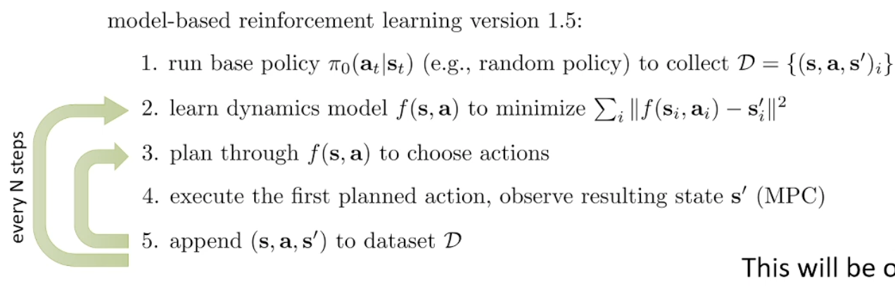
So this is quite like Imitation Learning where the first part can be formulated as a supervised learning problem. So it also need DAgger-like way to fix the distribution mismatch. In planning time, we can mix in MPC so the feedback loop is fast. So we got this:

Uncertainty

Model-based method may perform worse than the model free training. One of the reason is as we use NN, it overfits hard (the actual model space may be small).

If our model can model uncertainty, then sure it would still overfit, but it may say “this transition leads to high reward” but also says “…and I’m very uncertain about this prediction,” the planner can be conservative — it can avoid regions of state-action space where the model is unreliable.

Now, how can we get our network output uncertainty?

---

The following is from Claude Opus 4.6 with my edits:

Approach 1: Just use the logits?

If your model already outputs a categorical distribution (e.g. discretized next-state prediction), it’s tempting to just use the softmax probabilities as uncertainty. This is not a good idea for two reasons:

1. Calibration: Neural network softmax outputs are notoriously poorly calibrated — a model can output 0.99 confidence and still be wrong. Without additional calibration (temperature scaling, Platt scaling, etc.), the probabilities don’t faithfully reflect even the data noise.
2. Aleatoric only: Even if perfectly calibrated, softmax from a single model can only capture aleatoric uncertainty — the irreducible noise in $P(s_{t+1}|s_t,a_t)$. It fundamentally cannot capture epistemic uncertainty (uncertainty about the model itself). A single set of weights has no mechanism to say “I’ve never seen data like this” — it will just produce some output, often with high confidence, even on out-of-distribution inputs.

For model-based RL, epistemic uncertainty is exactly what we need. The planner exploits regions where the model is confidently wrong, and those are precisely the regions where epistemic uncertainty is high.

Now, we normally estimate $\arg {\max }_{\theta }\log p(D|\theta )$. If we an estimate the entropy of $p(\theta |D)$, we can get what we want.

Approach 2: Ensembles and Bayesian methods

The right approach is to maintain multiple plausible models and measure their disagreement.

Ensembles (e.g. bootstrap ensemble): Train $N$ models on different bootstrap samples of the data. In well-covered regions of state-action space, all $N$ models agree $\to$ low epistemic uncertainty. In sparse/OOD regions, each model overfit differently $\to$ high disagreement $\to$ high epistemic uncertainty. The variance across ensemble predictions is the uncertainty estimate.

Bagging is back! The approximation may be crute as the number of model is usually small. You may not need to do the data resampling, as NN retrained usually is sufficiently independent.

Bayesian neural networks: Maintain a posterior distribution over model parameters $P(\theta |\mathcal{D})$. The posterior predictive variance directly gives you epistemic uncertainty. Ensembles can be seen as a computationally cheaper approximation to this — each ensemble member is roughly a sample from an approximate posterior.

The key insight: this works because you’re sampling from the space of plausible explanations of the data. Disagreement between equally valid hypotheses is epistemic uncertainty by definition.

We can either penalize uncertain cases, or just do a simple averaging (softer).

Complex observations

Previously, we were assuming that the model state is relatively low-dimensional, but it can also be quite complex. For example, consider image:

• High dimensionality
• Redundancy
• Partial observability So we are dealing with a POMDP here.

One way to deal with it is to learn seperately $p(o_t|s_t)$ and $p(s_{t+1}|s_t,a_t)$ . That’s state space (latent space) models. $\begin{array}{rl}& \underset{\varphi }{\max }\frac{1}{N}\sum _{i=1}^N\sum _{t=1}^{T}E\left[\log p_{\varphi }({\mathbf{s}}_{t+1,i}|{\mathbf{s}}_{t,i},{\mathbf{a}}_{t,i})+\log p_{\varphi }({\mathbf{o}}_{t,i}|{\mathbf{s}}_{t,i})\right]\\ & \text{expectation w.r.t. }({\mathbf{s}}_t,{\mathbf{s}}_{t+1})\sim p({\mathbf{s}}_t,{\mathbf{s}}_{t+1}|{\mathbf{o}}_{1:T},{\mathbf{a}}_{1:T})\end{array}$ So we somehow need to know “where am I” to get started. We can also learn this posterior “encoder”: $q_{\psi }({\mathbf{s}}_t|{\mathbf{o}}_{1:t},{\mathbf{a}}_{1:t})$, in the simplest form it can be $q_{\psi }(s_t|o_t)$. If we have that and say it’s deterministic, we can take the expectation away and now it’s just ${\max }_{\varphi ,\psi }\frac{1}{N}{\sum }_{i=1}^N{\sum }_{t=1}^T\underset{\text{latent space dynamics}}{\underbrace{\log p_{\varphi }(g_{\psi }({\mathbf{o}}_{t+1,i})|g_{\psi }({\mathbf{o}}_{t,i}),{\mathbf{a}}_{t,i})}}+\underset{\text{image reconstruction}}{\underbrace{\log p_{\varphi }({\mathbf{o}}_{t,i}|g_{\psi }({\mathbf{o}}_{t,i}))}}+\underset{\text{reward model}}{\underbrace{\log p_{\varphi }(r_{t,i}|g_{\psi }({\mathbf{o}}_{t,i}))}}$

---

Now, we’ve assumed we are using planning once we got the state representation. We can also use a global policy for doing model-based RL with policies.

Just running back prop through state transitions would not work, since it’s the same issue as BPTT: vanishing or exploding gradient. So the common way to do this is just to treat the model as “fast simulator” for model free RL. Policy gradient might be more stable since it doesn’t require multiplying many Jacobians.

We want short rollouts since the learned model is approximate, which means distribution shift from the real world. The more we rely on it, the more we differentiate from it.

One of the general algorithms: Dyna