Kalman Filter

Kalman Filter is just Bayes Filter applied to a Gaussian linear setting.

Settings

First we have a state transition:

$$x_t=A_t{x}_{t-1}+B_t{u}_t+{\epsilon }_t$$

${\epsilon }_t$‘s mean is $0$ and the covariance is $R_t$.

Then we have the measurements:

$$z_t=C_t{x}_t+{\delta }_t$$

Again, measurement noise ${\delta }_t$ has $0$ mean and covariance $Q_t$.

The algorithm

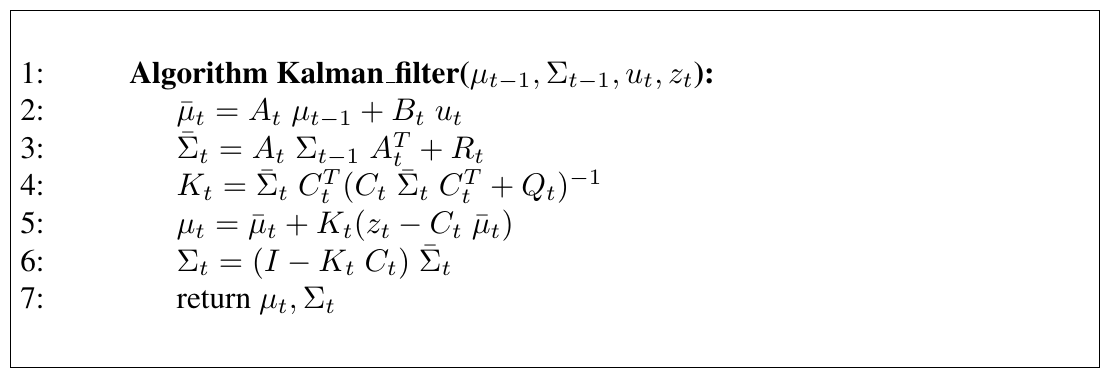
Here line 2 and 3 are calculating $\overline{bel}(x)$, while 5 and 6 are calculating $bel(x)$.

My own intuition

• ${\bar{\mu }}_t$: That’s easy from state transition formula
• ${\bar{\Sigma }}_t$: The original covariance goes through the linear formula, since the covariance is a quadratic matrix, we must have $A_t$ multiplied twice. Add the $R_t$ term for state transition noise.

On Kalman Gain

Kalman Gain: Let’s write this as

$$K_t=\frac{{\bar{\Sigma }}_t{C}_t^T}{C_t{\bar{\Sigma }}_t{C}_t^T+Q_t}$$

. That’s strange (and nobody pointed that out), cause obviously to make sense of it we need another $C_t$ there on the numerator part.

Let’s just say, $K_t$ is intuitively,

$$C_t^{-1}\ast \text{ratio of covariance}$$

. Of course there’s no guarantee that $C_t$ is invertible. But let’s just keep it that way.

Now onto the next formula. We compute the innovation: the difference of “real measurement” and “expected measurement”, $z_t-C_t{\hat{\mu }}_t$. Recall that $z_t=C_t{x}_t+{\delta }_t$. If we just multiply $C^{-1}$ to both side, we get $C_t^{-1}{z}_t=x_t+...$ . So here we are,

$$\begin{array}{rl}{\mu }_t& ={\bar{\mu }}_t+\text{ratio of covariance}(\alpha )\ast C_t^{-1}(z_t-C_t{\bar{\mu }}_t)\\ & =\alpha C^{-1}{z}_t+(1-\alpha ){\bar{\mu }}_t\end{array}$$

Voilà!

For the last one,

$${\Sigma }_t=(1-\alpha ){\bar{\Sigma }}_t$$

Why? If $\alpha \to 0$, that means measurement noise is too large, and we rely only on state update. If $\alpha \to 1$, measurement is so good we just need that, and we are super certain.

---

The derivation

The following notes are from Gauss-Markov Models, a supplementary material from 16-831, F14. It’s clearer than the version in the book Probabilistic Robotics.

Say we have a vector $x\sim \mathcal{N}(\mu ,\Sigma )$,

Linear transformation, $Ax$, is easier with moment parameterization. $Ax\sim \mathcal{N}(A\mu ,A\Sigma A^T)$.

Conditioning, getting $x_1|x_2$ from joint distribution $x$, is easier with natural parameterization. Note that conditioning is basically start from joint distribution and then treat $x_2$ as “known”.

$$x_1|x_2\sim \tilde{\mathcal{N}}(J_1-P_{12}{x}_2,P_{11})$$

If we want to multiply two likelihood function, $p(x|z)\sim p(z|x)p(x)$, then posterior can be simply computed by

$$x_1|z\sim \tilde{\mathcal{N}}(J_1+J_2,P_1+P_2)$$

Now with these in mind, we can have a gauss-markov model. I’m too tired now to repeat the stuff in the PDF. But the general idea is we do it in two steps. One prediction / rollup, one conditioning.

The former computes $p(x_t|z_1,...z_{t-1})$, and relies on $p(x_{t-1}=x|z_1,...z_{t-1})$. The latter is $p(x_t)|z_1,...,z_t$ and relies on the previous formula. The first step is easier in moment parameters, while the latter is easier in natural one.

If we use Sherman-Morrison-Woodbury formula and convert the natural parameterization to moment one, we get our familiar Kalman filter, which is an algorithm, not the underlying probabilistic model.

The "information" is Fisher information

The precision matrix $P={\Sigma }^{-1}$ in the natural parameterization is the Fisher Information about the state given the current belief. The measurement update $P_{\text{new}}=P_{\text{old}}+C^T{Q}^{-1}C$ is adding the Fisher information from the new observation. This is why conditioning is additive in natural parameters — Fisher information from independent observations adds. The Kalman filter achieves the Cramér-Rao bound: ${\Sigma }_t$ is the minimum-variance estimator, and ${\Sigma }_t^{-1}$ is the total accumulated Fisher information.