KL Divergence

Generated via Claude 4.6 Opus, resulted from a conversation.

---

The Kullback-Leibler divergence measures how one probability distribution $q$ differs from a reference distribution $p$:

$$D_{KL}(p|q)=\sum _{k}p(k)\log \frac{p(k)}{q(k)}=-\sum _{k}p(k)\log q(k)+\sum _{k}p(k)\log p(k)=H(p,q)-H(p)$$

It has several independent derivations. The most concrete starts from coding theory.

---

Coding Theory Motivation

Why start from coding theory for a quantity about probability distributions?

A probability distribution assigns beliefs over outcomes. The coding question asks: if you had to act on those beliefs — commit resources under uncertainty — how costly would it be? Code length is the most stripped-down version of that: allocating a finite resource (bits) based on how likely you think each outcome is.

$-\log p(k)$ keeps appearing not because we care about bits per se, but because the logarithm is the unique function that converts multiplicative probability structure into additive cost structure while respecting independence. Coding theory is just the cleanest context where that becomes concrete — you can point at a literal string of bits and say “this is what your wrong beliefs cost you.”

You could skip coding entirely: define $D_{KL}$ by formula, prove non-negativity, show uniqueness from axioms. That’s mathematically complete but unmotivated. The coding interpretation gives physical intuition for why each piece is there — why $p(k)$ weights, why $\log$, why the ratio $p/q$.

The Setup: Encoding Messages

Suppose we need to transmit a sequence of symbols (events, classes, outcomes) over a channel. Each symbol is drawn from some distribution $p$. We want to assign a binary code to each symbol — shorter codes for frequent symbols, longer codes for rare ones.

For example, if we have four symbols with equal probability $1/4$, we need 2 bits each: 00, 01, 10, 11. But if symbol A occurs 50% of the time, we’d prefer to give it a shorter code.

The Kraft Inequality: What Constrains Code Lengths

For a code to be uniquely decodable (no codeword is a prefix of another), the code lengths ${\ell }_k$ must satisfy:

$$\sum _k{2}^{-{\ell }_k}\le 1$$

This is the Kraft inequality. It’s a hard constraint from the structure of binary prefix codes — it limits how many short codewords you can have. If you make one code shorter, others must get longer.

Optimal Code Lengths → Entropy

Given this constraint, what code lengths minimize the expected cost ${\sum }_{k}p(k),{\ell }_k$? This is a constrained optimization problem. Using Lagrange multipliers, the solution is:

$${\ell }_k^{\ast }=-\log p(k)$$

Plugging back in, the minimum achievable expected code length is:

$$\sum _{k}p(k),{\ell }_k^{\ast }=-\sum _{k}p(k)\log p(k)=H(p)$$

This is entropy — not defined axiomatically, but derived as the solution to “minimize expected code length subject to Kraft.” That’s Shannon’s source coding theorem: no lossless code beats $H(p)$, and codes exist that come arbitrarily close.

Note

Fractional bits $-\log p(k)$ is generally not an integer. Practical codes like Huffman coding round to integers (achieving average length between $H(p)$ and $H(p)+1$). Arithmetic coding gets arbitrarily close to $H(p)$ by encoding sequences jointly rather than symbol-by-symbol. The theorem is an asymptotic statement about what’s achievable in principle.

Using the Wrong Code → Cross-Entropy

Now suppose reality follows $p$, but we design our code for distribution $q$. By the same Kraft argument, the optimal code lengths for $q$ are $-\log q(k)$. But symbols still occur with frequency $p(k)$. The expected code length becomes:

$$\sum _{k}p(k)(-\log q(k))=H(p,q)$$

This is cross-entropy. The $p(k)$ weighting doesn’t change — reality is still $p$ — we’ve just plugged in the wrong code lengths.

The Excess Cost → KL Divergence

The difference between what we pay and what we could have paid:

$$H(p,q)-H(p)=\sum _{k}p(k)\log \frac{p(k)}{q(k)}=D_{KL}(p|q)$$

KL divergence is the extra bits per symbol you pay for using $q$ instead of $p$.

"Surprise" is an interpretation, not the foundation

$-\log p(k)$ is often introduced as the “surprise” of event $k$, with entropy defined as “expected surprise.” This is a useful interpretation — the quantity is indeed zero for certain events, large for rare ones, and additive for independent events. But these properties aren’t axioms chosen because “surprise should work this way.” They’re consequences of $-\log p(k)$ being the optimal code length under the Kraft inequality. “Surprise” is a name we give to the result after the fact.

---

Other Derivations

Hypothesis Testing

Given $N$ i.i.d. samples from $p$, the expected log-likelihood ratio between $p$ and $q$ is:

$$\frac{1}{N}\sum _{i=1}^N\log \frac{p(x_i)}{q(x_i)}\stackrel{N\to \infty }{\to }{D}_{KL}(p|q)$$

KL divergence is the expected evidence per sample in favor of $p$ over $q$ when $p$ is true. This connects to Stein’s lemma: $D_{KL}$ governs the exponential decay rate of Type II error in hypothesis testing.

Axiomatic Uniqueness

KL divergence can be characterized as essentially the unique divergence satisfying:

• $D(p|q)\ge 0$ with equality iff $p=q$
• Additivity over independent variables
• Invariance under sufficient statistics (the data processing inequality)

This is formalized through Csiszár’s work on $f$-divergences.

---

Connection to Riemannian Geometry

For two nearby distributions $p_{\theta }$ and $p_{\theta +d\theta }$ on the Statistical Manifold, KL divergence to second order is:

$$D_{KL}(p_{\theta }|p_{\theta +d\theta })\approx \frac{1}{2}d{\theta }^{T}F(\theta )d\theta$$

where $F(\theta )$ is the Fisher Information matrix. The Fisher metric is the local quadratic approximation of KL divergence — this is how information geometry derives the Riemannian structure of probability space from KL divergence, not the other way around.

This is why the Natural Gradient — which uses $F(\theta {)}^{-1}\nabla J$ — is the steepest descent direction in the geometry induced by KL divergence rather than Euclidean distance.

---

Properties

• Non-negative: $D_{KL}(p|q)\ge 0$ (Gibbs’ inequality), with equality iff $p=q$
• Asymmetric: $D_{KL}(p|q)\ne D_{KL}(q|p)$ in general — it is not a true metric
• Not a distance: violates triangle inequality and symmetry
• Additive: for independent variables, $D_{KL}(p_1{p}_2|q_1{q}_2)=D_{KL}(p_1|q_1)+D_{KL}(p_2|q_2)$

---

The following comes from blog post:

• Approximating KL Divergence by John Schulman
• KL Divergence for Machine Learning by Dibya Ghosh, who at the time was Sergey’s student.

Discussed with Claude Sonnet 4.6

---

Forward vs. Reverse KL: Geometric Intuition

KL divergence is asymmetric — $D_{\text{KL}}(q|p)\ne D_{\text{KL}}(p|q)$ — and the two directions have fundamentally different optimization behavior. The names forward and reverse are convention-dependent, so the behavior is the thing to hold onto.

Consider fitting an approximate distribution $q$ to a target $p$.

In the illustration, $P$ is the blue one, bimodal, and $Q_{\theta }$ the normal one, orange.

Minimizing $D_{\text{KL}}(p|q)$ — sampling from $p$, penalizing where $p$ has mass that $q$ misses:

$$D_{\text{KL}}(p|q)={\mathbb{E}}_{x\sim p}\left[\log \frac{p(x)}{q(x)}\right]$$

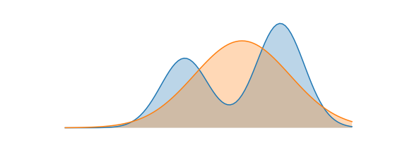A good approximation under this objective satisfies: wherever $p$ has high probability, $q$ must also have high probability. The mechanism is that wherever $p(x)>0$ but $q(x)\approx 0$, the term $\log (p/q)$ blows up — so $q$ is forced away from zero there. If $p$ is bimodal, $q$ will spread between both modes rather than miss one entirely, even if the result fits neither mode well. This is mass-covering (or mean-seeking) behavior.

Minimizing $D_{\text{KL}}(q|p)$ — sampling from $q$, penalizing where $q$ has mass that $p$ doesn’t support:

$$D_{\text{KL}}(q|p)={\mathbb{E}}_{x\sim q}\left[\log \frac{q(x)}{p(x)}\right]$$

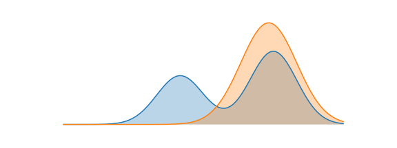A good approximation under this objective satisfies: wherever $q$ has high probability, $p$ must also have high probability. The mechanism is that wherever $q(x)>0$ but $p(x)\approx 0$, the term $\log (q/p)$ blows up — so $q$ is afraid to put mass outside $p$‘s support. If $p$ is bimodal, $q$ will snap to one mode and ignore the other. The entropy term in the expansion prevents $q$ from collapsing to a point; the typical behavior is to find the widest mode of $p$ and mimic it exactly. This is mode-seeking behavior.

Gradient scaling intuition

The functional derivative with respect to $q(x)$ makes the asymmetry precise:

$$\frac{\partial }{\partial q(x)}{D}_{\text{KL}}(p\Vert q)=-\frac{p(x)}{q(x)}\frac{\partial }{\partial q(x)}{D}_{\text{KL}}(q\Vert p)=\log \frac{q(x)}{p(x)}+1$$

The $p/q$ term diverges as $q(x)\to 0$ — this is the mechanism behind mass-covering. The $\log (q/p)$ term grows only logarithmically, which is why mode-seeking exerts much weaker pressure toward coverage. Source: Max Shen’s blog

What Access Do You Need?

The choice of direction is often constrained by what you have access to, not just preference:

• $D_{\text{KL}}(p|q)$ requires samples from $p$ — you evaluate $\log q(x)$ at those samples. This is the supervised learning setting: you have a dataset drawn from the true distribution.
• $D_{\text{KL}}(q|p)$ requires evaluating $p(x)$ pointwise — you sample from $q$ and score those samples under $p$. This is the RL setting: you can’t sample optimal trajectories, but you can score any trajectory via reward.

Connections to Supervised Learning and RL

Supervised learning minimizes forward KL. Given a dataset of samples $x_i\sim p_{\text{data}}$, minimizing Cross Entropy loss over a model $q_{\theta }$ is identical to minimizing $D_{\text{KL}}(p_{\text{data}}|q_{\theta })$, since the entropy of $p_{\text{data}}$ is a constant:

$$D_{\text{KL}}(p|q_{\theta })=\underset{\text{cross-entropy}}{\underbrace{{\mathbb{E}}_p[-\log q_{\theta }(x)]}}-\underset{\text{constant}}{\underbrace{{\mathbb{E}}_p[-\log p(x)]}}$$

This covers classification (cross-entropy loss), regression (MSE = NLL of a Gaussian), and maximum likelihood estimation generally.

RL minimizes reverse KL. In the control-as-inference framing (Sergey’s work), optimal trajectories have probability $\propto \exp ({\sum }_t{r}_t)$. We can’t sample from this distribution directly, but we can evaluate it. Minimizing $D_{\text{KL}}(q_{\theta }|p_{\text{optimal}})$ over a policy $q_{\theta }$ recovers the max-entropy RL objective — which is exactly why reverse KL is the natural regularizer in RLHF and PPO. You want the actor to stay within the reference’s support, not cover all of it.

---

Monte Carlo Estimation of KL

When $p$ and $q$ are high-dimensional (e.g., distributions over sequences), computing $D_{\text{KL}}(q|p)={\mathbb{E}}_{x\sim q}[\log q/p]$ analytically is intractable. We only have pointwise access to $\log p(x)$ and $\log q(x)$ at sampled $x$. So we need a Monte Carlo estimator.

Define $r=p(x)/q(x)$ (the density ratio at a sample). Three natural estimators exist, each with different bias/variance properties.

The Three Estimators

$$k_1=-\log r=\log \frac{q}{p}{k}_2=\frac{1}{2}(\log r{)}^2{k}_3=(r-1)-\log r$$

All three are trying to estimate the same quantity $D_{\text{KL}}(q|p)$, but they trade off differently.

$k_1$ is the direct definition rewritten: ${\mathbb{E}}_q[k_1]=D_{\text{KL}}(q|p)$ exactly (unbiased). But individual samples can be negative (since $\log r$ has no sign constraint), while the true KL is always non-negative. This sign-flipping creates high variance — the estimator is correct on average but noisy sample by sample.

$k_2$ fixes the sign problem by squaring: every sample is non-negative. But ${\mathbb{E}}_q[k_2]\ne D_{\text{KL}}(q|p)$ in general — it is biased. The bias is small when $q\approx p$, and grows as the distributions diverge.

$k_3$ achieves the best of both: it is unbiased like $k_1$ and always non-negative like $k_2$.

Numerical Comparison (from Schulman)

$q=\mathcal{N}(0,1)$, $p=\mathcal{N}(0.1,1)$, true $\mathrm{KL}=0.005$:

Estimator	bias / true KL	std / true KL
$k_1$	0	20
$k_2$	0.002	1.42
$k_3$	0	1.42

With larger divergence ($p=\mathcal{N}(1,1)$, true $\mathrm{KL}=0.5$):

Estimator	bias / true KL	std / true KL
$k_1$	0	2
$k_2$	0.25	1.73
$k_3$	0	1.70

$k_3$ dominates: unbiased with low variance in the small-KL regime, and still competitive when KL is large. The bias of $k_2$ becomes serious once $q$ and $p$ are far apart.

$k_3$ is not always the right choice

The numerical comparison above makes $k_3$ look strictly better, but the choice of estimator depends on how KL is used in code — not just value estimation quality. Xihuai Wang (2025) shows that when KL is used as a differentiable loss term (direct backprop), naively backpropagating through $k_3$ on-policy gives the forward KL gradient, not reverse — the wrong direction. And when KL is used as reward shaping (stop-gradient), $k_3$ introduces a bias term equal to $-\nabla D_{\text{KL}}(p|q)$ into the policy gradient update. In both cases $k_1$ or $k_2$ may be more appropriate depending on the setup. See Choosing KL Estimators in RL for the full analysis.

Notably, $k_3$ is the one that’s being used in GRPO.

---

Why $k_3$ Works: Three Perspectives

1. Control Variate

Any quantity with zero expectation under $q$ can be added to $k_1$ without introducing bias. The only natural zero-mean term here is $r-1=p(x)/q(x)-1$, since ${\mathbb{E}}_q[r]=\int q\cdot (p/q),dx=1$. So for any $\lambda$:

$$k_1+\lambda (r-1)=-\log r+\lambda (r-1)$$

is still unbiased. The question is what $\lambda$ minimizes variance. The optimal $\lambda$ depends on $p$ and $q$ and has no closed form. But a simple argument fixes $\lambda =1$: since $\log$ is concave, $\log x\le x-1$ for all $x>0$, so setting $\lambda =1$ guarantees the estimator is non-negative everywhere. Positivity alone substantially reduces variance.

2. f-Divergence and Second-Order Universality

An f-divergence is any functional of the form:

$$D_f(p|q)={\mathbb{E}}_{x\sim q}\left[f\left(\frac{p(x)}{q(x)}\right)\right]$$

for a convex $f$ with $f(1)=0$. KL corresponds to $f(x)=-\log x$. The expectation of $k_2$ is the f-divergence with $f(x)=\frac{1}{2}(\log x{)}^2$. These are different divergences, but a key fact is:

All f-divergences agree to second order near $p=q$

For any differentiable convex $f$, a parametric family $p_{\theta }$ near $p_0$:

D_f(p_0 | p_\theta) = \frac{f''(1)}{2} ,\theta^\top F \theta + O(\theta^3) $$ where $F$ is the [[Fisher information]] matrix. Normalizing so $f''(1) = 1$, all f-divergences look like $\frac{1}{2}\theta^\top F\theta$ locally — the same quadratic.

Both $f(x)=-\log x$ (KL) and $f(x)=\frac{1}{2}(\log x{)}^2$ ($k_2$‘s expectation) satisfy $f^{\prime \prime }(1)=1$. So $k_2$‘s expectation is a faithful local surrogate for KL whenever $q\approx p$. The bias only becomes visible when the distributions separate enough for third-order terms to matter.

3. Bregman Divergence

The deepest perspective. A Bregman divergence generated by a convex function $\varphi$ is:

$$B_{\varphi }(x|y)=\varphi (x)-\varphi (y)-{\varphi }^{\prime }(y)(x-y)$$

This measures the gap between $\varphi (x)$ and the tangent plane to $\varphi$ at $y$, evaluated at $x$. Since $\varphi$ is convex, it lies above all its tangent lines, so $B_{\varphi }\ge 0$ always — and the gap vanishes only when $x=y$.

Now let $\varphi (x)=-\log x$, and evaluate $B_{\varphi }(r|1)$:

$$B_{\varphi }(r|1)=-\log r-(-\log 1)-\underset{=-1}{\underbrace{{\varphi }^{\prime }(1)}}(r-1)=-\log r+(r-1)=k_3$$

So $k_3$ is exactly the Bregman divergence of $\varphi (x)=-\log x$, between the ratio $r$ and the equilibrium point $r=1$ (where $p=q$). Non-negativity is not a clever trick — it falls out immediately from convexity of $\varphi$.

KL itself is also a Bregman divergence

$D_{\text{KL}}(q|p)=B_{-H}(q|p)$ where $\varphi =-H$ is the negative entropy, acting on probability vectors. So both KL and $k_3$ are Bregman divergences — one between distributions, one between scalar values of the ratio $r$. The non-negativity and the quadratic shrinking near $r=1$ both descend from the same convexity argument.

The General Recipe

For any f-divergence with convex $f$, subtracting the tangent at $r=1$ gives an always-positive, unbiased estimator:

$$f(r)-f^{\prime }(1)(r-1)$$

This is $B_f(r|1)$ — the Bregman divergence of $f$ at the equilibrium. For $D_{\text{KL}}(p|q)$, use $f(x)=x\log x$ (which has $f^{\prime }(1)=1$), giving the estimator $r\log r-(r-1)$.

Target	$f(x)$	Estimator
$D_{\text{KL}}(q\Vert p)$	$-\log x$	$(r-1)-\log r=k_3$
$D_{\text{KL}}(p\Vert q)$	$x\log x$	$r\log r-(r-1)$

The Unifying Inequality

All three perspectives trace back to one fact:

$$\log x\le x-1\text{for all }x>0,\text{ with equality iff }x=1$$

This is just concavity of $\log$, or equivalently convexity of $-\log$. It is also the same inequality used to prove $D_{\text{KL}}\ge 0$ via Jensen’s inequality. The non-negativity of KL and the non-negativity of $k_3$ share the same root.